CapsNet architecture for MNIST

I recently wrote an article explaining the intuitive idea of capsules proposed by Geoffrey Hinton and colleagues which created a buzz in the deep learning community. In that article, I explained in simple terms the motivation behind the idea of capsules and its (minimal) mathematical formalism. It is highly recommended that you read that article as a prerequisite to this one. In this article, I would like to explain the specific CapsNet architecture proposed in the same paper which managed to achieve state-of-the-art performance on the MNIST digit classification.

capsnet

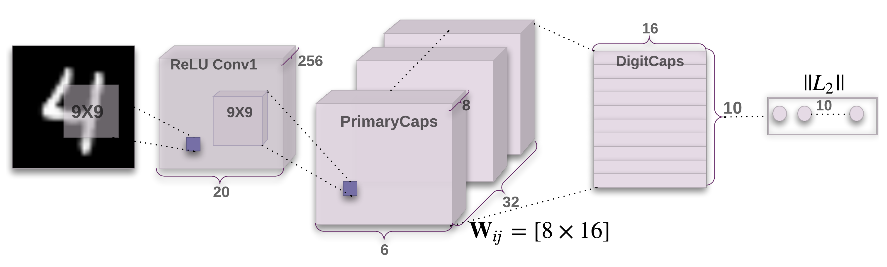
The architecture diagram in the paper is pretty much a good representation of the model. But I’ll still try to make things easier by explaining it part-by-part. If you have gone through my previous article, you should have least complication in understanding the architecture. The CapsNet architecture is composed of 3 layers and they are as follows:

1. First convolutional layer: This is an usual convolutional layer. In case of MNIST digits, a single digit image of shape 28 x 28 is convolved by 256 kernels of shape 9 x 9. In the paper, the authors decided not to zero-pad the inputs to keep the feature map dimensions same. So, the output of this layer is 256 feature maps/activation maps of shape 20 x 20. ReLU has been used as the activation function.

layer_1

2. Second convolutional layer or the PrimaryCaps layer: For a clear understanding, I am breaking this layer into two parts:

   • This is just another convolutional layer which applies 256 convolutional kernels of shape 9 x 9 (no zero-padding as the first one) and stride 2 which produces 256 activation maps of 6 x 6.

   • The output of the second convolutional layer (6 x 6 x 256) is interpreted as a set of 32 “capsule activation maps” with capsule dimension 8. By “capsule activation map” I mean an activation map of capsules instead of scalar-neurons. The below diagram depicts these capsule activation maps quite clearly. So, we have a total of 6*6*32 = 1152 capsules (each of dimension 8) which are then flattened on a capsule level to make an array of 1152 capsules. Finally, each capsule is applied through a vector non-liearity.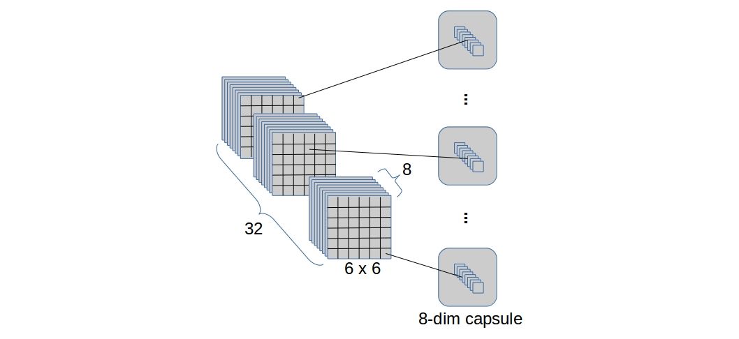

3. A capsule-to-capsule layer or DigitCaps layers: This layer is exactly what I explained in the last part of my previous post. The 1152 (lower level) capsules are connected to 10 (higher levels) capsules which has a total of 1152*10 = 11520 weight matrices \(W_{ij}\). The 10 higher level capsules (of dimension 16) represent the 10 final “digit/class entities”. Vector non-linearity is again applied on these capsules so that the lengths can be treated as probability of existence of a particular digit entity. This layer also has the “dynamic routing” in it.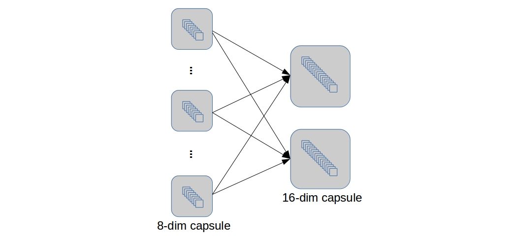

To summarize, an image of shape 28 x 28 when passed through the CapsNet, will produce a set of 10 capsule activations (each of dimension 16) each of which represents the “explicit pose parameters” of the digit entity (the class) it is associated with.

The loss function

The objective function used for training the CapsNet is well known to the machine learning community. It is a popular variation of the “Hinge Loss”, namely “Squared Hinge loss” or “L2-SVM loss”. I do not intend to explain the loss function in detail, you may want to check this instead. The basic idea is to calculate the lengths (probability of existence - between 0 and 1) of the 10 digit capsules and maximizing the one corresponding to the label while minimizing the rest of them.

The loss for the \(i^{th}\) sample is \(\displaystyle{ L^{(i)} = \sum_{j \in \mathbb{C}} \left[ y_j^{(i)} max(0, m^+- \|\|v_j^{(i)}\|\| )^2 + \lambda (1-y_j^{(i)}) max(0, \|\|v_j^{(i)}\|\|-m^-)^2 \right] }\)

where, \(\mathbb{C}\) is the set of classes, \(\|\|v_j^{(i)}\|\|\) is the length of the digit capsule activation of class \(j\) for the \(i^{th}\) sample and \(y^{(i)}\) is the “one hot” encoding of the label of sample \(i\). \(m^+\) and \(m^-\) are the margins of the margin loss which have been taken to be 0.9 and 0.1 respectively. \(\lambda = 0.5\) decays the loss for the absent digit classes.

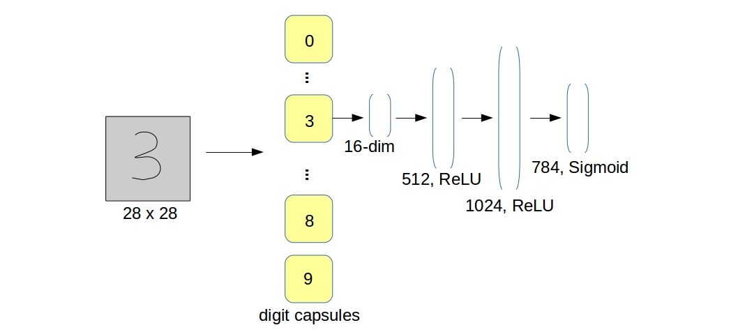
A regularizer

The authors of the paper decided to use a regularizer in the training process which is basically a “decoder network” that reconstructs the input digit images from the (16 dimensional) activity vector of its corresponding class-capsule. It is a simple 3-layer fully connected network with ReLU activations in the 2 hidden layers and Sigmoid in the last layer. The reconstructed vector is the flattened image of size 784. The dimensions of the layers of the decoder network are shown in the figure below.

decoder

Tensorflow implementation

Link to my full implementation: https://github.com/dasayan05/capsule-net-TF

Let’s dive into some code. Things will make sense as we move on. I am using python and the tensorflow library to create a static computation graph that represents the CapsNet architecture.

Let’s start by defining the placeholders - a batch of MNIST digit images (of shape batch x image_w x image_h x image_c) and the one hot encoded labels (of shape batch x n_class). An extra (batch) dimension on axis 0 will always be there as we intend to do batch learning.

x = tf.placeholder(tf.float32, shape=(None,image_w,image_h,image_c), name='x')
y = tf.placeholder(tf.float32, shape=(None,n_class), name='y')

The shape of x has been chosen to be compatible with the convolutional layer API (tf.layers.conv2d). The two successive conv2ds are as follows

conv1_act = tf.layers.conv2d(x, filters=256, kernel_size=9, strides=1, padding='VALID',
    kernel_initializer=tf.contrib.layers.xavier_initializer(),
    activation=tf.nn.relu,
    use_bias=True, bias_initializer=tf.initializers.zeros) # shape: (B x 20 x 20 x 256)

primecaps_act = tf.layers.conv2d(conv1_act, filters=8*32, kernel_size=9, strides=2, padding='VALID',
            kernel_initializer=tf.contrib.layers.xavier_initializer(),
            activation=tf.nn.relu,
            use_bias=True, bias_initializer=tf.initializers.zeros) # shape: (B x 6 x 6 x 256)

Now that we have 256 primecaps activation maps (of shape 6 x 6), we have to arrange them in a set of 32 “capsule activation maps” with capsules dimension 8. So we tf.reshape and tf.tile it. The tiling is required for simplifying some future computation.

primecaps_act = tf.reshape(primecaps_act, shape=(-1, 6*6*32, 1, 8, 1)) # shape: (B x 1152 x 1 x 8 x 1)
# 10 is for the number of classes/digits
primecaps_act = tf.tile(primecaps_act, [1,1,10,1,1]) # shape: (B x 1152 x 10 x 8 x 1)

Next, we apply vector non-linearity (the squashing function proposed in the paper)

def squash(x, axis):
    # x: input tensor
    # axis: which axis to squash
    # I didn't use tf.norm() here to avoid mathamatical instability
    sq_norm = tf.reduce_sum(tf.square(x), axis=axis, keep_dims=True)
    scalar_factor = sq_norm / (1 + sq_norm) / tf.sqrt(sq_norm + eps)
    return tf.multiply(scalar_factor, x)

# axis 3 is the capsule dimension axis
primecaps_act = squash(primecaps_act, axis=3) # squashing won't change shape

As we have total 1152 capsule activations (all squashed), we are now ready to create the capsule-to-capsule layer or the DigitCaps layer. But we need the affine transformation parameters (\(W_{ij}\)) to produce the “prediction vectors” for all \(i\) and \(j\).

W = tf.get_variable('W', dtype=tf.float32, initializer=tf.initializers.random_normal(stddev=0.1),
    shape=(1, 6*6*32, 10, 8, 16)) # shape: (1, 1152, 10, 8, 16)

# bsize: batch size
W = tf.tile(W, multiples=[bsize,1,1,1,1]) # shape: (B x 1152 x 10 x 8 x 16)

Calculate the prediction vectors. Applying tf.matmul on W and primecaps_act will matrix-multiply the last two dimensions of each tensor. The last two dimensions of W and primecaps_act are 16 x 8 (because of transpose_a=True option) and 8 x 1 respectively.

u = tf.matmul(W, primecaps_act, transpose_a=True) # shape: (B x 1152 x 10 x 16 x 1)
# reshape it for routing
u = tf.reshape(tf.squeeze(u), shape=(-1, 6*6*32, 16, 10)) # shape: (B x 1152 x 16 x 10)

Now, its time for the routing. We declare the logits \(b_{ij}\) as tf.constant so that they re-initialize on every sess.run() call or in other words, on every batch. After R iterations, we get the final \(v_j\).

# bsize: batch size
bij = tf.constant(zeros((bsize, 6*6*32, 10), dtype=float32), dtype=tf.float32) # shape: (B x 1152 x 10)

for r in range(R):
    # making sure sum_cij_over_j is one
    cij = tf.nn.softmax(bij, dim=2) # shape: (B x 1152 x 10)

    s = tf.reduce_sum(u * tf.reshape(cij, shape=(-1, 6*6*32, 1, 10)),
        axis=1, keep_dims=False) # shape: (B x 16 x 10)

    # v_j = squash(s_j); vector non-linearity
    v = squash(s, axis=1) # shape: (B x 16 x 10)

    if r < R - 1: # bij computation not required at the end
        # reshaping v for further multiplication
        v_r = tf.reshape(v, shape=(-1, 1, 16, 10)) # shape: (B x 1 x 16 x 10)

        # the 'agreement'
        uv_dot = tf.reduce_sum(u * v_r, axis=2)

        # update logits with the agreement
        bij += uv_dot

That’s all for the forward pass. All that is left is defining the loss and attaching an optimizer to it. We calculate the classification loss (the squared-hinge loss) after computing the lengths of the 10 digit/class capsules.

v_len = tf.sqrt(tf.reduce_sum(tf.square(v), axis=1) + eps) # shape: (B x 10)

MPlus, MMinus = 0.9, 0.1
# this is very much similar to the actual mathematical formula I showed earlier
l_klass = y * (tf.maximum(zeros((1,1),dtype=float32), MPlus-v_len)**2) + \
        lam * (1-y) * (tf.maximum(zeros((1,1),dtype=float32), v_len-MMinus)**2)

# take mean loss over the batch
loss = tf.reduce_mean(l_klass)

# add an optimizer of your choice
optimizer = tf.train.AdamOptimizer()
train_step = optimizer.minimize(loss)

I am not showing the reconstruction loss here in this article but my actual implementation does have the reconstruction loss. You should refer to it for any other confusion.