---
config:
  look: handDrawn
  themeVariables:
    fontSize: 22px
---
graph TD
    subgraph P1["Part I: Stat/Prob"]
        direction LR
        a1["Random<br/>variables"]
        a2[Distributions]
        a3["Parameter<br/>estimation"]
        a4["Bayesian<br/>thinking"]
        a5["Joint &<br/>conditional"]
        a6["Hypothesis<br/>testing"]
        a1 ~~~ a2 ~~~ a3 ~~~ a4 ~~~ a5 ~~~ a6
    end

    subgraph P2["Part II: Spatial Stat."]
        direction LR
        b1["Point<br/>patterns"]
        b2["Spatial<br/>graphs"]
        b3["Neighbourhood<br/>structure"]
        b4["Spatial<br/>autocorrelation"]
        b5["Generative<br/>models"]
        b1 ~~~ b2 ~~~ b3 ~~~ b4 ~~~ b5
    end

    P1 == "builds on" ==> P2
Mathematical and Statistical Inference
7MBM1008 - AI for Imaging and Spatial Data
Dr. Ayan Das
November 20, 2026
Self Introduction

What do I do ?
- Computer Scientist
- Work in Generative AI
- AI for Healthcare/Dentistry
- Focused on Image modalities
- Bit of fundamentals AI research
Module Information
Statistics for Spatial Data.
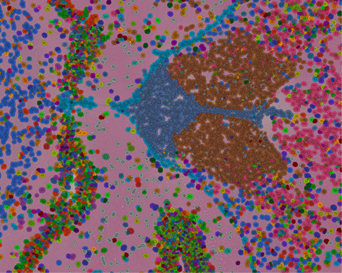
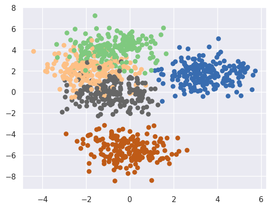
Similarities
- Modelling collective behaviour
- Recognising patterns in data
- Dealing with inherent randomness
Lecture Outline
- Part I: fast-paced recap
- Part II: slower, in depth
- More intuition, less rigorous math
- lots of interactive diagrams
- sometimes simplified for illustration
Statistics
“.. the science of collecting, analyzing, organizing and interpreting data to make decision under uncertainty.”
Random Variable
Numerical description of a random phenomenon.
 Flipping a coin
Textual Description
\(X\) = “outcome of flipping a coin” / “heads or tails on top when flipped ?”
Known Possible Outcomes (Sample Space \(\Omega\))
\(\Omega = \{ \text{heads}, \text{tails} \}\)
Numerical Mapping, \(X: \Omega \rightarrow \mathbb{Z}\)
Every outcome is mapped to a number, e.g. \(\text{Heads} \rightarrow 1, \quad \text{Tails} \rightarrow 0\)
Trials/Observations/Measurements
Each time the outcome is unpredictable, but strictly within its sample space
\(\{ 0, 1, 1, 0, 0, 1, 0, 1, 1, 0, 0, \ldots, 1 \}\)
Random Variable
Numerical description of a random phenomenon.
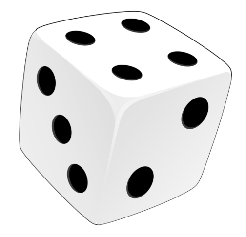 Rolling a die.
Textual Description
\(X\) = “outcome of rolling a die” / “number of dots on top when rolled”
Known Possible Outcomes (Sample Space \(\Omega\))
\(\Omega = \{ \text{Rolling a 1}, \text{Rolling a 2}, \ldots, \text{Rolling a 6} \}\)
Numerical Mapping, \(X: \Omega \rightarrow \mathbb{Z}\)
Every outcome is mapped to a number, e.g.
\(\text{Rolling a 1} \rightarrow 1, \quad \text{Rolling a 2} \rightarrow 2, \quad \ldots, \quad \text{Rolling a 6} \rightarrow 6\)
Trials/Observations/Measurements
Each time the outcome is unpredictable, but strictly within its sample space.
\(\{ 1, 2, 3, 4, 5, 6, 1, 2, 3, 4, 5, 6, \ldots, 1 \}\)
Question for you
I again rolled a die 50 times ..
array([2, 3, 4, 1, 1, 1, 5, 4, 3, 5, 1, 5, 1, 2, 1, 3, 5, 1, 4, 2, 5, 1,
       1, 4, 2, 2, 1, 1, 2, 1, 2, 1, 4, 1, 3, 2, 1, 1, 5, 1, 2, 1, 1, 2,
       2, 1, 1, 1, 1, 1])
Probability Distribution
How likely is each outcome of a random variable ?
For discrete RVs, its functional form is the “Probability Mass Function” or PMF.
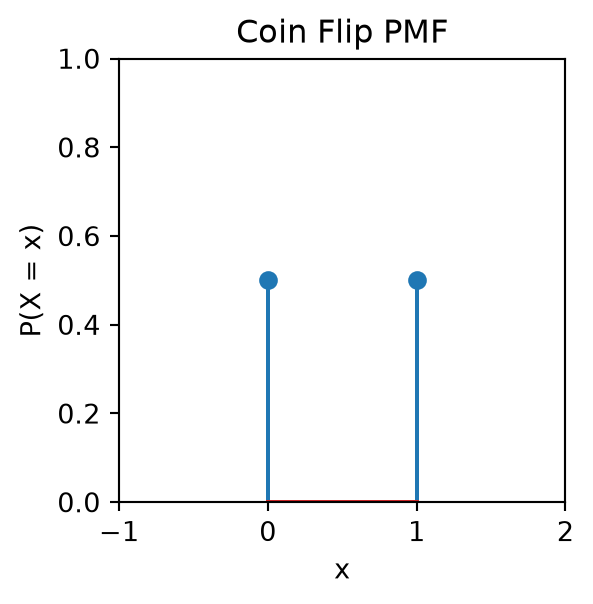
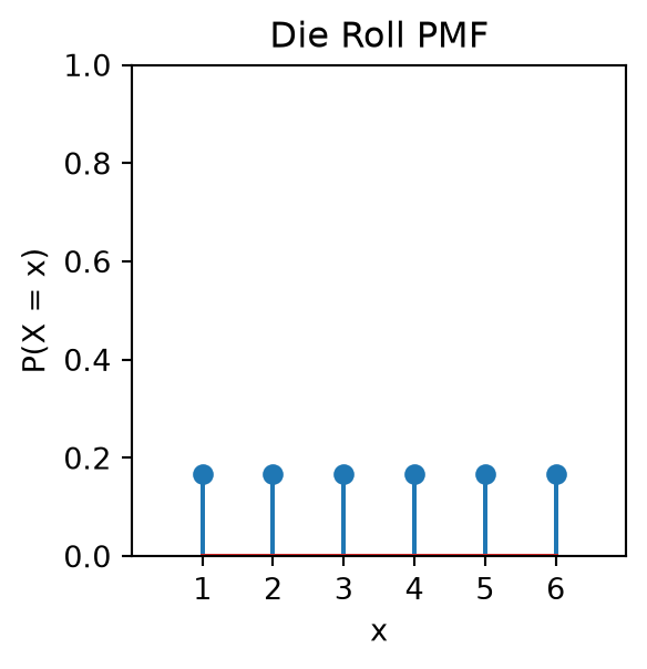
\(P(X = x)\) or \(p(x)\) or \(p_X(x)\) reads as “the probability that \(X\) takes the value \(x\)”.
Properties of Probability
- \(P(X = x) \in [0.0, 1.0]\) for all \(x \in \Omega\)
- \(\sum_{x \in \Omega} P(X = x) = 1\)
Different PMFs for same RV
Let’s consider the die roll example.
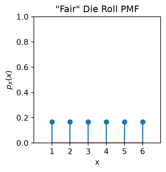
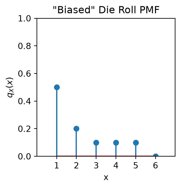
The \(\sim\) Notations
\(X \sim p_X(x)\) reads as “\(X\) is distributed according to \(p_X(x)\)”. Similarly, \(X \sim q_X(x)\) reads as “\(X\) is distributed according to \(q_X(x)\)”.
Unknown parameters
We assumed the probabilities for the ‘biased’ die. But, in reality, we don’t know the probabilities.
\[ X \sim q_X(x; \theta) \]
\[ \text{where we try to find } \theta = [\theta_1, \theta_2, \theta_3, \theta_4, \theta_5, \theta_6] \]
We have access to \(n\) observations
\[ \{ x_1 = 1, x_2 = 2, x_3 = 1, x_4 = 1, x_5 = 5, \ldots, x_n = 1 \} \]
Statistical Inference
Estimating \(\theta\) from the observations is the goal of “statistical inference” \[ \theta \approx \mathrm{Inference}(\{ x_1, x_2, \ldots, x_n \}) \]
Estimating PMF from Observations
PMF is often unknown, and all we have are observations.
rolls = {
  const pmf = [0.5, 0.2, 0.1, 0.1, 0.1, 0.0];
  const cdf = pmf.map((_, i) => pmf.slice(0, i + 1).reduce((a, b) => a + b, 0));
  const sample = () => { const u = Math.random(); return cdf.findIndex(c => u < c) + 1; };
  return Array.from({length: num_observations}, sample);
}
md`[${rolls.join(", ")}]`
Histogram
\[ H(x) = \text{# of times } x\text{ appears in observations} \]
Normalised Histogram (Probabilities)
\[ \hat{q}_X(x) = \frac{H(x)}{\text{# of observations}} \]
// histogram of rolls
Plot.plot({
  width: 400, height: 220,
  x: { label: "x", domain: [1,2,3,4,5,6], tickFormat: d => d },
  y: { label: "H(x)", domain: [0, 30] },
  marks: [
    Plot.barY([1,2,3,4,5,6].map(v => ({ x: v, y: rolls.filter(r => r === v).length })),
      { x: "x", y: "y", fill: "steelblue" }),
    Plot.text([1,2,3,4,5,6].map(v => ({ x: v, y: rolls.filter(r => r === v).length })),
      { x: "x", y: "y", text: d => String(d.y), dy: -6, fontSize: 12 }),
    Plot.ruleY([0])
  ]
})
// normalised histogram of rolls
Plot.plot({
width: 400, height: 220,
x: { label: "x", domain: [1,2,3,4,5,6], tickFormat: d => d },
y: { label: "p(x)", domain: [0, 1] },
marks: [
Plot.barY([1,2,3,4,5,6].map(v => ({ x: v, y: rolls.filter(r => r === v).length / rolls.length })),
{ x: "x", y: "y", fill: "tomato" }),
Plot.text([1,2,3,4,5,6].map(v => ({ x: v, y: rolls.filter(r => r === v).length / rolls.length })),
{ x: "x", y: "y", text: d => d.y.toFixed(2), dy: -6, fontSize: 12 }),
Plot.ruleY([0])
]
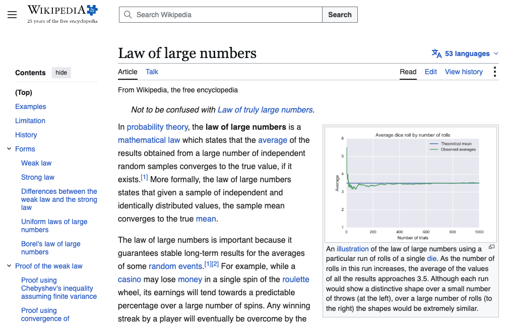
})More observations, better estimates
Another example: Event Count
Textual Description
\(X\) = “number of events occurring in a fixed interval”
Known Possible Outcomes (Sample Space \(\Omega\))
\(X \in \{0, 1, 2, 3, \ldots\}\)
Numerical Mapping, \(X: \Omega \rightarrow \mathbb{N}\)
Every outcome is already numerical, so \(X: \Omega \to \{0, 1, 2, 3, \ldots\}\).
A popular choice for modelling event counts is the Poisson distribution \[ P(X = k) = \frac{e^{-\lambda} \lambda^k}{k!} \]
{
  void seed; // re-run when button is clicked

  // Sample n ~ Poisson(lambda) using Knuth's algorithm
  function samplePoisson(lam) {
    const L = Math.exp(-lam);
    let k = 0, p = 1;
    do { k++; p *= Math.random(); } while (p > L);
    return k - 1;
  }

  const n = samplePoisson(lambda * 3);
  const pts = Array.from({length: n}, () => ({x: Math.random() * 3}));

  return Plot.plot({
    width: 380,
    height: 100,
    marginTop: 35,
    marginBottom: 40,
    x: {domain: [0, 3], label: "Fixed interval →", ticks: 3},
    y: {axis: null, domain: [-0.5, 0.5]},
    marks: [
      Plot.ruleY([0], {stroke: "#888", strokeWidth: 1.5}),
      Plot.dot(pts, {x: "x", y: 0, r: 7, fill: "steelblue", stroke: "white", strokeWidth: 1.5, opacity: 0.85})
    ]
  });
}
{
// Poisson PMF: P(X=k) = e^{-λ} λ^k / k!
const kMax = Math.max(20, lambda * 3);
const data = Array.from({length: kMax + 1}, (_, k) => {
let logP = -lambda + k * Math.log(lambda);
for (let i = 2; i <= k; i++) logP -= Math.log(i);
return {k, p: Math.exp(logP)};
});
return Plot.plot({
width: 380,
height: 160,
x: {label: "k", tickFormat: d => d},
y: {label: "P(X = k)", grid: true},
marks: [
Plot.barY(data, {x: "k", y: "p", fill: "steelblue", opacity: 0.8}),
Plot.ruleY([0])
]
});
}(Continuous) Random Variable
 Height of a person
Textual Description
\(X\) = “height of a person (in cm)”
Known Possible Outcomes (Sample Space \(\Omega\))
\(X \in [0, \infty)\) (Theoretically)
\(X \in [0, 270]\) (Practically)
Numerical Mapping
The outcomes are already numerical, so \(X: \Omega \to [0, 270]\).
Trials/Observations/Measurements
We can measure the height of multiple persons, and each time the outcome is unpredictable, but strictly within its sample space.
\(\{ 192.91, 169.49, 164.93, 171.01, 179.19, 184.12, 165.93, 164.26, \ldots \}\)
Probability Density Function (PDF)
Analogous to PMF (for discrete RVs), but for continuous RVs.
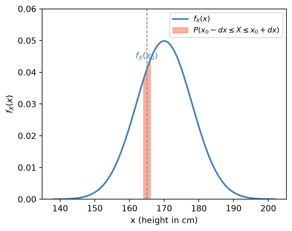
The PDF \(f_X(x)\) is “density”, not “probability”.
\[ P(x - dx \leq X \leq x + dx) \approx f_X(x) \cdot dx \]
Inference from observations
Estimating PDF, aka “density estimation” problem.
Histogram
\[ H(x) = \text{# of observations in bin } [x - dx, x + dx] \]
Normalised Histogram (Probabilities)
\[ \hat{f}_X(x) = \frac{H(x)}{\text{total # of observations}} \]
// histogram of observed heights
Plot.plot({
  width: 400, height: 260,
  x: { label: "height (cm)", domain: [130, 210] },
  y: { label: "count" },
  marks: [
    Plot.rectY(observed_heights, Plot.binX({ y: "count" }, { x: d => d, thresholds: 10, fill: "steelblue" })),
    Plot.dot(observed_heights, { x: d => d, y: 0, fill: "tomato", r: 4, fillOpacity: 0.7 }),
    Plot.ruleY([0])
  ]
})
// normalised histogram of observed heights
Plot.plot({
width: 400, height: 260,
x: { label: "height (cm)", domain: [130, 210] },
y: { label: "density" },
marks: [
Plot.rectY(observed_heights, Plot.binX({ y: "proportion" }, { x: d => d, thresholds: 10, fill: "tomato", fillOpacity: 0.6 })),
Plot.lineY(observed_heights, Plot.binX({ y: "proportion" }, { x: d => d, thresholds: 10, stroke: "tomato", strokeWidth: 2 })),
Plot.dotY(observed_heights, Plot.binX({ y: "proportion" }, { x: d => d, thresholds: 10, fill: "tomato", r: 3 })),
Plot.dot(observed_heights, { x: d => d, y: 0, fill: "steelblue", r: 4, fillOpacity: 0.7 }),
Plot.ruleY([0])
]
})Assume a parametric form
Restricting the possibilities.
Assume a gaussian density for the height distribution, i.e. \(X \sim N(\mu, \sigma^2)\). \[ f_X(x; \theta = (\mu, \sigma)) = \frac{1}{\sigma \sqrt{2\pi}} e^{-\frac{(x - \mu)^2}{2\sigma^2}} \]
Model
Simplifying assumption we make as statisticians. We restrict the possible densities to a specific family.
Trade-off
We simplify the problem, reducing the number of parameters to estimate, but we loose flexibility. In fact, we could be wrong in our assumption.
// plot the assumed density
{
  const xs = Array.from({length: 300}, (_, i) => mu - 4*sigma + i * (8*sigma / 299));
  const gaussPDF = x => (1 / (sigma * Math.sqrt(2 * Math.PI))) * Math.exp(-0.5 * ((x - mu) / sigma) ** 2);
  const data = xs.map(x => ({ x, y: gaussPDF(x) }));
  return Plot.plot({
    width: 400, height: 260,
    x: { label: "x", domain: [100, 230] },
    y: { label: "f(x; μ, σ)", domain: [0, 0.1] },
    marks: [
      Plot.lineY(data, { x: "x", y: "y", stroke: "steelblue", strokeWidth: 2 }),
      Plot.dot(observed_heights, { x: d => d, y: 0, fill: "tomato", r: 2, fillOpacity: 0.7 }),
      Plot.ruleY([0])
    ]
  });
}
A wrong model/assumption
Heights from two different countries, but we assume a gaussian PDF.
bimodal_heights = {
  const sample = (mu, sigma) => mu + sigma * Math.sqrt(-2 * Math.log(Math.random())) * Math.cos(2 * Math.PI * Math.random());
  const group1 = Array.from({length: 100}, () => sample(170, 5));
  const group2 = Array.from({length: 100}, () => sample(140, 5));
  return [...group1, ...group2].map(v => parseFloat(v.toFixed(2)));
}

bimodal_heights
// plot the bimodal heights histogram with points overlaid on x-axis
Plot.plot({
width: 400, height: 260,
x: { label: "height (cm)", domain: [100, 210] },
y: { label: "count" },
marks: [
Plot.rectY(bimodal_heights, Plot.binX({ y: "count" }, { x: d => d, thresholds: 15, fill: "steelblue", fillOpacity: 0.6 })),
Plot.dot(bimodal_heights, { x: d => d, y: 0, fill: "tomato", r: 3, fillOpacity: 0.7 }),
Plot.ruleY([0])
]
})// plot the assumed gaussian density with points overlaid on x-axis
{
const xs = Array.from({length: 300}, (_, i) => mu_ - 4*sigma_ + i * (8*sigma_ / 299));
const gaussPDF = x => (1 / (sigma_ * Math.sqrt(2 * Math.PI))) * Math.exp(-0.5 * ((x - mu_) / sigma_) ** 2);
const data = xs.map(x => ({ x, y: gaussPDF(x) }));
return Plot.plot({
width: 400, height: 260,
x: { label: "x", domain: [100, 210] },
y: { label: "f(x; μ, σ)", domain: [0, 0.1] },
marks: [
Plot.lineY(data, { x: "x", y: "y", stroke: "steelblue", strokeWidth: 2 }),
Plot.dot(bimodal_heights, { x: d => d, y: 0, fill: "tomato", r: 2, fillOpacity: 0.7 }),
Plot.ruleY([0])
]
});
}Available PDF models
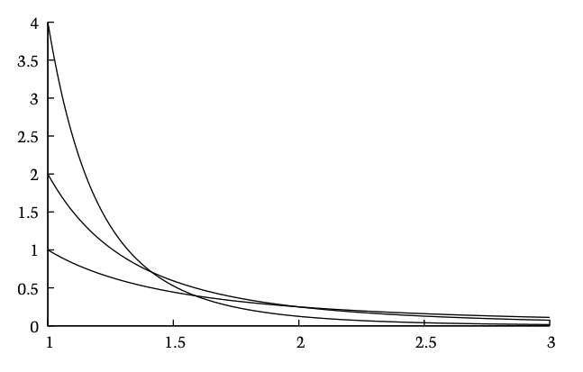
Pareto Distribution
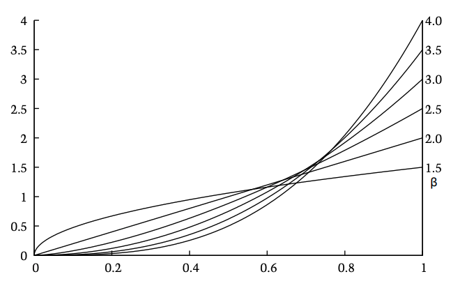
Pearson Type IX Distribution
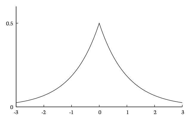
Laplace Distribution
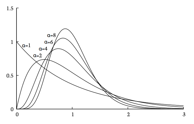
Gamma Distribution
Maximum Likelihood Estimation (MLE)
Given a parametric model \(f_X(x; \theta)\), we want to find the parameter \(\theta\) that maximizes the likelihood of the observed data.
\[ \hat{\theta} = \arg\max_{\theta} L(\theta) = \arg\max_{\theta} \prod_{x_i \in D} f_X(x_i; \theta) \]
we achieve this by iteratively updating \(\theta\) using gradient ascent
\[ \theta_{t+1} = \theta_t + \eta \nabla_\theta L(\theta_t) \]
The realm of Machine Learning
- MLE is fundamental to many ML algorithms, e.g. linear regression, logistic regression, naive bayes, etc.
- Deep Learning is essentially MLE with neural networks as the parametric model, with ‘backpropagation’ for optimization.
- The backbone behind modern Generative AI like LLM, Diffusion Models, etc.
Kernel Density Estimation (KDE)
‘Non-parametric’ density estimation technique.
\[ \begin{aligned} &f_{\mathrm{KDE}}(x; h) = \frac{1}{n} \sum_{x_i \in D} K_h(x - x_i) \\ &= \frac{1}{n} \sum_{x_i \in D} f_{\mathrm{Gaussian}}(x; \mu = x - x_i, \sigma = h) \end{aligned} \]
Kernel
- A kernel is a smooth non-negative function.
- The kernel is often a Gaussian, but others possible too.
- The kernel is centered at each observation \(x_i\).
- The bandwidth \(h\) controls the smoothness of the final density.
// plot the KDE using a Gaussian kernel with bandwidth h
// show 5 points on the x-axis and put individual gaussians in dotted line
{
  const pts = [1.5, 2.1, 4.0, 5.5, 8.5];
  const n = pts.length;
  const h = bandwidth;
  const gaussK = (x, xi) => Math.exp(-0.5 * ((x - xi) / h) ** 2) / (h * Math.sqrt(2 * Math.PI));

  const xMin = -1, xMax = 10;
  const xs = Array.from({length: 300}, (_, i) => xMin + i * (xMax - xMin) / 299);

  const kernelLines = pts.flatMap(xi =>
    xs.map(x => ({ x, y: gaussK(x, xi) / n, xi: String(xi) }))
  );

  const kdeData = xs.map(x => ({
    x,
    y: pts.reduce((s, xi) => s + gaussK(x, xi), 0) / n
  }));

  return Plot.plot({
    width: 400, height: 260,
    x: { label: "x", domain: [xMin, xMax] },
    y: { label: "f_KDE(x; h)", domain: [0, 0.55] },
    marks: [
      Plot.line(kernelLines, {
        x: "x", y: "y", z: "xi",
        stroke: "steelblue", strokeWidth: 1.2,
        strokeDasharray: "4,3", strokeOpacity: 0.55
      }),
      Plot.line(kdeData, {
        x: "x", y: "y",
        stroke: "tomato", strokeWidth: 2.5
      }),
      Plot.dot(pts.map(xi => ({ x: xi, y: 0 })), {
        x: "x", y: "y",
        fill: "steelblue", r: 6, fillOpacity: 0.85
      }),
      Plot.ruleY([0])
    ]
  });
}
Downsides
- Complexity grows with number of observations.
- Bandwidth is hyperparameter. Not always easy to choose.
Important Definitions
Mean (Expectation)
The “center of mass” of the distribution.
\[ \mathbb{E}[X] = \mathbb{E}_{f_X(x)}[X] = \int_{\Omega} x f_X(x) dx \]
Variance
The “spread” of the distribution.
\[ \begin{aligned} \text{Var}_{f_X(x)}[X] &= \mathbb{E}[(X - \mathbb{E}[X])^2] \\ &= \int_{\Omega} (x - \mathbb{E}[X])^2 f_X(x) dx \end{aligned} \]
Joint Distribution
\[ P(x, y) \]
captures the relationship between two random variables.
Conditional Distribution
\[ P(X | Y = y) \]
is the distribution of \(X\) given that \(Y\) takes a specific value \(y\).
Bayes’ Theorem: A Primer
We observe data \(X\). We want the hidden parameter \(\theta\) of the model behind it.
Forward and inverse
\[ \begin{aligned} \theta \ &\longrightarrow\ X &&: \ p(X \mid \theta) \ \text{(likelihood)} \\ \theta \ &\longleftarrow\ X &&: \ p(\theta \mid X) \ \text{(posterior)} \end{aligned} \]
- \(\theta\): model parameter, hidden
- \(X\): observation, what we measure
Bayes’ theorem
\[ p(\theta \mid X) = \frac{p(X \mid \theta)\, p(\theta)}{p(X)} \ \propto\ p(X \mid \theta)\, p(\theta) \]
Likelihood \(p(X \mid \theta)\)
How well \(\theta\) explains \(X\). The same quantity MLE maximises.
Prior \(p(\theta)\)
What we believe about \(\theta\) before seeing \(X\).
Posterior \(p(\theta \mid X)\)
What we believe after seeing \(X\).
Evidence \(p(X) = \int p(X \mid \theta)\, p(\theta)\, d\theta\)
Only a normaliser, it does not depend on \(\theta\).
The solver
\[ p(\theta \mid X) = \texttt{Solver}\big(X,\ p(X \mid \theta),\ p(\theta)\big) \]
- In: data \(X\), a likelihood model we can evaluate, a prior (no \(p(X)\) needed)
- Out: the whole posterior distribution, not a single value. Compare \(\hat\theta = \texttt{MLE}\big(X,\ p(X \mid \theta)\big)\), which returns one number.
(Continuous) Random “Vector”
More than one random variable, i.e. a vector of random variables.
Textual Description
\(C = \text{spatial location of a cell} = \begin{bmatrix} \text{x-coordinate} \\ \text{y-coordinate} \end{bmatrix}\)
Known Possible Outcomes (Sample Space \(\Omega\))
\(\Omega = [0, \mathrm{width}] \times [0, \mathrm{height}]\)
Numerical Mapping
\(C: \Omega \to [0, \mathrm{width}] \times [0, \mathrm{height}]\).
Trials/Observations/Measurements
Observations are now vectors e.g. \(\begin{bmatrix} 3.2 \\ 7.1 \end{bmatrix}, \begin{bmatrix} 6.5 \\ 4.8 \end{bmatrix}, \ldots\).
hw_data = {
  const n = 20;
  const mu1 = 5, mu2 = 5;
  const l11 = 1.5, l21 = 1.05, l22 = 1.071;
  const randn = () => Math.sqrt(-2 * Math.log(Math.random())) * Math.cos(2 * Math.PI * Math.random());
  return Array.from({length: n}, () => {
    const z1 = randn(), z2 = randn();
    return { x1: parseFloat((mu1 + l11 * z1).toFixed(2)),
             x2: parseFloat((mu2 + l21 * z1 + l22 * z2).toFixed(2)) };
  });
}

Plot.plot({
  width: 380, height: 320,
  x: { label: "x", domain: [0, 10] },
  y: { label: "y", domain: [0, 10] },
  marks: [
    Plot.dot(hw_data, { x: "x1", y: "x2", fill: "steelblue", r: 5, fillOpacity: 0.7 }),
    Plot.frame()
  ]
})
2D parametric Density Model
The 2D Gaussian PDF is defined as
\[ f_C(\bar{c}; \theta = (\bar{\mu}, \Sigma)) = \frac{1}{2\pi |\Sigma|^{1/2}} \exp\Big(-\frac{1}{2} (\bar{c} - \bar\mu)^T \Sigma^{-1} (\bar{c} - \bar\mu)\Big) \]
\[ \text{where, } \bar\mu = \begin{bmatrix} \mu_1 \\ \mu_2 \end{bmatrix}, \quad \Sigma = \begin{bmatrix} \sigma_1^2 & \rho \sigma_1 \sigma_2 \\ \rho \sigma_1 \sigma_2 & \sigma_2^2 \end{bmatrix} \]
viewof mu1 = Inputs.range([0, 10], {value: 5, step: 0.1, label: "μ₁"})
viewof mu2 = Inputs.range([0, 10], {value: 5, step: 0.1, label: "μ₂"})
viewof sigma1 = Inputs.range([0.2, 3], {value: 1.5, step: 0.1, label: "σ₁"})
viewof sigma2 = Inputs.range([0.2, 3], {value: 1.5, step: 0.1, label: "σ₂"})
viewof rho = Inputs.range([-0.9, 0.9], {value: 0.7, step: 0.05, label: "ρ"})
// plot the 2D Gaussian PDF (isocontour plot) using sliders for mu1, mu2, sigma1, sigma2, rho
// and overlay the observed data points
{
const pdf2d = (x, y) => {
const denom = 1 - rho ** 2;
const z = ((x - mu1) / sigma1) ** 2
- 2 * rho * ((x - mu1) / sigma1) * ((y - mu2) / sigma2)
+ ((y - mu2) / sigma2) ** 2;
return Math.exp(-z / (2 * denom)) / (2 * Math.PI * sigma1 * sigma2 * Math.sqrt(denom));
};
return Plot.plot({
width: 380, height: 320,
x: { label: "x", domain: [0, 10] },
y: { label: "y", domain: [0, 10] },
color: { scheme: "Blues" },
marks: [
Plot.raster({ fill: pdf2d, x1: 0, x2: 10, y1: 0, y2: 10 }),
Plot.contour({ value: pdf2d, x1: 0, x2: 10, y1: 0, y2: 10,
stroke: "white", strokeOpacity: 0.7, strokeWidth: 1.2 }),
Plot.dot(hw_data, { x: "x1", y: "x2", fill: "tomato", r: 3, fillOpacity: 0.8 }),
Plot.frame()
]
});
}2D Kernel Density Estimation
Non-parametric density estimation for 2D data.
// plot the 2D KDE of the observed data using Gaussian kernel with bandwidth h
{
  const h = bandwidth2d;
  const n = hw_data.length;
  const gaussK = (x, xi) => Math.exp(-0.5 * ((x - xi) / h) ** 2) / (h * Math.sqrt(2 * Math.PI));
  const kde2d = (x, y) => {
    let sum = 0;
    for (const pt of hw_data) sum += gaussK(x, pt.x1) * gaussK(y, pt.x2);
    return sum / n;
  };
  return Plot.plot({
    width: 400, height: 340,
    x: { label: "x", domain: [0, 10] },
    y: { label: "y", domain: [0, 10] },
    color: { scheme: "YlOrRd" },
    marks: [
      Plot.raster({ fill: kde2d, x1: 0, x2: 10, y1: 0, y2: 10 }),
      Plot.contour({ value: kde2d, x1: 0, x2: 10, y1: 0, y2: 10,
                     stroke: "white", strokeOpacity: 0.7, strokeWidth: 1.2 }),
      Plot.dot(hw_data, { x: "x1", y: "x2", fill: "black", r: 3, fillOpacity: 0.85 }),
      Plot.frame()
    ]
  });
}
\[ \begin{aligned} &f_{\mathrm{KDE}}(\bar{c}; h) = \frac{1}{n} \sum_{\bar{c}_i \in D} K_h(\bar{c} - \bar{c}_i) \\ &= \frac{1}{n} \sum_{\bar{c}_i \in D} f_{\mathrm{Gaussian2D}}(\bar{c}; \mu = \bar{c} - \bar{c}_i, \Sigma = h \mathrm{I}) \end{aligned} \]
Significant or Pure luck ?
Remember the die I rolled 50 times ..
Observation
14 ones in 50 rolls
The skeptic’s claim
“The die is fair”: \(P(X = 1) = \frac{1}{6}\)
So we expect only \(50 \times \frac{1}{6} \approx 8.3\) ones.
The question
If the die were fair, how surprising is 14 ones ?
// 10 x 5 grid of rolls, ones highlighted
Plot.plot({
  width: 420, height: 230, margin: 10,
  x: {axis: null, domain: [-0.5, 9.5]},
  y: {axis: null, domain: [-0.5, 4.5]},
  marks: [
    Plot.dot(ht_grid, {x: "x", y: "y", r: 15,
      fill: d => d.one ? "tomato" : "#e8eef5",
      stroke: d => d.one ? "tomato" : "steelblue", strokeOpacity: 0.6}),
    Plot.text(ht_grid, {x: "x", y: "y", text: "v", fontSize: 14, fontWeight: 600,
      fill: d => d.one ? "white" : "#333"})
  ]
})
Hypothesis Testing: Ask the simulator
Pretend the die is fair, and let luck play out many times.
Assume the skeptic is right
Fair die, \(P(X = 1) = \frac{1}{6}\)
Simulate
Roll 50 times, count the ones. Repeat many times.
ht_null = {
  void ht_resim; // re-run when button is clicked
  return Array.from({length: 100}, () => {
    let c = 0;
    for (let i = 0; i < 50; i++) if (Math.random() < 1 / 6) c++;
    return c;
  });
}

// fraction of simulations for each possible count 0..25
ht_counts = {
  const h = new Array(26).fill(0);
  for (const v of ht_null) if (v <= 25) h[v]++;
  return h.map((c, k) => ({k, f: c / ht_null.length}));
}

// measured mean and standard deviation of the simulated counts
ht_stats = {
  const N = ht_null.length;
  const m = ht_null.reduce((a, v) => a + v, 0) / N;
  const sd = Math.sqrt(ht_null.reduce((a, v) => a + (v - m) ** 2, 0) / (N - 1));
  return {m, sd};
}

ht_gauss = x => Math.exp(-0.5 * ((x - ht_stats.m) / ht_stats.sd) ** 2) / (ht_stats.sd * Math.sqrt(2 * Math.PI))
{
const curve = Array.from({length: 261}, (_, i) => -0.5 + i * 0.1).map(x => ({x, y: ht_gauss(x)}));
// right tail: from the observed count up to the end of the axis
const n = Math.round((25.5 - ht_obs) / 0.1);
const tail = Array.from({length: n + 1}, (_, i) => ht_obs + i * 0.1).map(x => ({x, y: ht_gauss(x)}));
return Plot.plot({
width: 520, height: 300,
x: {label: "# of ones in 50 rolls of a FAIR die", domain: [-0.5, 25.5]},
y: {label: "fraction of simulations", grid: true},
marks: [
Plot.rectY(ht_counts, {x1: d => d.k - 0.5, x2: d => d.k + 0.5, y: "f",
fill: "steelblue", fillOpacity: 0.35, stroke: "white"}),
Plot.areaY(tail, {x: "x", y: "y", fill: "orange", fillOpacity: 0.55}),
Plot.lineY(curve, {x: "x", y: "y", stroke: "darkorange", strokeWidth: 2.5}),
Plot.ruleX([ht_obs], {stroke: "tomato", strokeWidth: 2.5}),
Plot.ruleY([0])
]
});
}p-value
Probability of a result at least this extreme, if the skeptic is right. Usual threshold: \(p < 0.05\) → “significant”, reject the claim.
“Spatial” Statistics
Analysing data with spatial coordinates, to understand how location shapes patterns, relationships and variation.
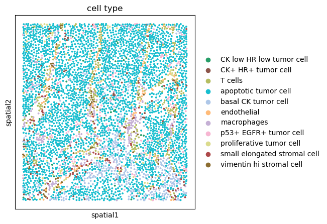
Some realistic examples1
Motivating further algorithms in spatial statistics.
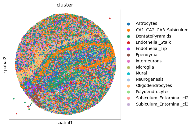
Some realistic examples1
Motivating further algorithms in spatial statistics.
Complete Spatial Randomness (CSR)
The 2D version of poisson “event count” explained earlier.
poisson = lam => {
  // Knuth's algorithm
  const L = Math.exp(-lam);
  let k = 0, p = 1;
  do { k++; p *= Math.random(); } while (p > L);
  return k - 1;
}

randn = () => Math.sqrt(-2 * Math.log(1 - Math.random())) * Math.cos(2 * Math.PI * Math.random())

// CSR: n points, independent and uniform in the unit square
gen_csr = n => Array.from({length: n}, () => ({x: Math.random(), y: Math.random()}))

// clustered: Gaussian blobs around random parent locations
gen_clustered = (n, spread) => {
  const k = Math.max(3, Math.round(n / 10));
  const parents = gen_csr(k);
  return Array.from({length: n}, () => {
    const c = parents[Math.floor(Math.random() * k)];
    let x, y;
    do {
      x = c.x + spread * randn();
      y = c.y + spread * randn();
    } while (x < 0 || x > 1 || y < 0 || y > 1);
    return {x, y};
  });
}

// regular: random points, rejected if too close to an existing one
// strength in (0, 1]: minimum distance as a fraction of the densest-packing scale
gen_regular = (n, strength) => {
  let r = strength * 0.75 / Math.sqrt(n);
  const pts = [];
  let fails = 0;
  while (pts.length < n) {
    const p = {x: Math.random(), y: Math.random()};
    if (pts.every(q => (p.x - q.x) ** 2 + (p.y - q.y) ** 2 >= r * r)) {
      pts.push(p);
      fails = 0;
    } else if (++fails > 2000) {
      r *= 0.95; // too crowded, relax the minimum distance
      fails = 0;
    }
  }
  return pts;
}

// plain scatter of points in the unit square
scatter_unit = (pts, color, size = 300) => Plot.plot({
  width: size, height: size,
  x: {domain: [0, 1], axis: null},
  y: {domain: [0, 1], axis: null},
  marks: [
    Plot.dot(pts, {x: "x", y: "y", fill: color, r: 3.5, fillOpacity: 0.8}),
    Plot.frame()
  ]
})
Spatial Poisson Process
Events fall independently and uniformly, at an average density of \(\lambda\) per unit area.
\[ P(N(A) = k) = \frac{e^{-\lambda |A|} (\lambda |A|)^k}{k!} \] where \(N(A)\) = number of points in region \(A\), and \(|A|\) = its area.
The null model
Given the number of points, their locations have “No spatial pattern” – means CSR.
Plot.plot({
  width: 340, height: 340,
  x: {domain: [0, 3], label: "Region A, |A| = 3 × 3 = 9", ticks: 3},
  y: {domain: [0, 3], axis: null},
  marks: [
    Plot.ruleX([1], {stroke: "gray", strokeDasharray: "2,4", strokeOpacity: 0.5}),
    Plot.ruleY([1], {stroke: "gray", strokeDasharray: "2,4", strokeOpacity: 0.5}),
    Plot.dot(csr_pts, {x: "x", y: "y", fill: "steelblue", r: 4.5, fillOpacity: 0.8, stroke: "white", strokeWidth: 1}),
    Plot.frame()
  ]
})
Clustered, random or regular?
Same number of points, very different organisation.
rk_n = 45
rk_rmax = 0.25
rk_step = 0.005
rk_nsteps = Math.round(rk_rmax / rk_step)
rk_types = ["clustered", "random", "regular"]
rk_colors = ["tomato", "steelblue", "seagreen"]

// three patterns in the unit square, their K(r) curves, and one randomly chosen "focal" point each
rk_seed = 200
rk_data = {
  const rnd = cen_rng(rk_seed), orig = Math.random;
  Math.random = rnd; // fixed seed, so the slide looks the same every time
  const sets = {}, focals = {};
  try {
    sets.clustered = gen_clustered(rk_n, 0.1);
    sets.random = gen_csr(rk_n);
    sets.regular = gen_regular(rk_n, 1);
    for (const t of rk_types) focals[t] = Math.floor(rnd() * rk_n);
  } finally {
    Math.random = orig;
  }
  const out = {};
  for (const type of rk_types) {
    const pts = sets[type], n = pts.length;
    // every ordered pair i != j: distance and translation edge-correction weight 1 / (area of window ∩ shifted window)
    const pairs = [];
    for (let i = 0; i < n; i++) for (let j = 0; j < n; j++) {
      if (i === j) continue;
      const dx = Math.abs(pts[i].x - pts[j].x), dy = Math.abs(pts[i].y - pts[j].y);
      pairs.push({d: Math.hypot(dx, dy), w: 1 / ((1 - dx) * (1 - dy))});
    }
    pairs.sort((a, b) => a.d - b.d);
    // K(r) = |A| / (n (n - 1)) * sum of weights of the pairs closer than r, with |A| = 1
    const curve = [];
    let k = 0, acc = 0;
    for (let s = 0; s <= rk_nsteps; s++) {
      const r = s * rk_step;
      while (k < pairs.length && pairs[k].d <= r) acc += pairs[k++].w;
      curve.push({type, s, r, K: acc / (n * (n - 1))});
    }
    out[type] = {pts, curve, focal: focals[type]};
  }
  return out;
}

rk_curves = rk_types.flatMap(t => rk_data[t].curve)
rk_ymax = 1.05 * Math.max(...rk_curves.map(d => d.K), Math.PI * rk_rmax ** 2)

// the three patterns in one square, with a circle of radius r around each focal point
rk_scene = (r, size) => {
  const dots = [], rings = [], centres = [];
  for (const type of rk_types) {
    const {pts, focal} = rk_data[type], f = pts[focal];
    pts.forEach((p, i) => dots.push({
      type, x: p.x, y: p.y,
      inside: i !== focal && Math.hypot(p.x - f.x, p.y - f.y) <= r
    }));
    centres.push({type, x: f.x, y: f.y});
    if (r > 0) for (let a = 0; a <= 64; a++) rings.push({
      type, x: f.x + r * Math.cos(2 * Math.PI * a / 64), y: f.y + r * Math.sin(2 * Math.PI * a / 64)
    });
  }
  return Plot.plot({
    width: size, height: size, margin: 4,
    x: {domain: [0, 1], axis: null},
    y: {domain: [0, 1], axis: null},
    color: {domain: rk_types, range: rk_colors},
    marks: [
      Plot.line(rings, {x: "x", y: "y", z: "type", stroke: "type", fill: "type", fillOpacity: 0.10, strokeWidth: 2, curve: "linear-closed", clip: true}),
      Plot.dot(dots, {x: "x", y: "y", fill: "type", r: 3.5, fillOpacity: d => d.inside ? 0.75 : 0.35}),
      Plot.dot(centres, {x: "x", y: "y", fill: "type", r: 6, fillOpacity: 1}),
      Plot.frame()
    ]
  });
}

// K(r) curves, drawn only up to the current radius, against the CSR reference pi r^2
rk_kplot = (r, w, h) => {
  const s = Math.round(r / rk_step);
  const shown = rk_curves.filter(d => d.s <= s);
  const csr = Array.from({length: rk_nsteps + 1}, (_, i) => ({r: i * rk_step, K: Math.PI * (i * rk_step) ** 2}));
  return Plot.plot({
    width: w, height: h, marginLeft: 48,
    x: {domain: [0, rk_rmax], label: "radius r"},
    y: {domain: [0, rk_ymax], label: "K(r)", grid: true},
    color: {domain: rk_types, range: rk_colors, legend: true},
    marks: [
      Plot.line(csr, {x: "r", y: "K", stroke: "gray", strokeDasharray: "5,4", strokeWidth: 1.5}),
      Plot.text([{r: rk_rmax, K: Math.PI * rk_rmax ** 2}], {x: "r", y: "K", text: ["CSR: πr²"], fill: "gray", textAnchor: "end", dy: 14, dx: -4}),
      Plot.line(shown, {x: "r", y: "K", stroke: "type", strokeWidth: 3}),
      Plot.dot(shown.filter(d => d.s === s), {x: "r", y: "K", fill: "type", r: 5, stroke: "white", strokeWidth: 1.5}),
      Plot.frame()
    ]
  });
}
Ripley’s K function
Average number of other points within distance \(r\) of a point, per unit density.
\[ \hat K(r) = \frac{|A|}{n(n-1)} \sum_{i \neq j} \mathbf{1}(d_{ij} \le r) \qquad\quad K_{\text{CSR}}(r) = \pi r^2 \]
Above the dashed line: clustered. Below it: regular.
Circle = the count around one point; curve = average over all points (edge-corrected).
rt_n = 80      // points in the fixed set
rt_m = 40      // points in each random subset (a random half)
rt_r = 0.1     // the one radius we test at
rt_csr = Math.PI * rt_r ** 2   // K(r) under CSR, about 0.031
rt_seed = 79   // chosen so that uniform points happen to look a bit lumpy

// the fixed point set: uniform in the unit square, generated once from a fixed seed
rt_pts = {
  const orig = Math.random;
  Math.random = cen_rng(rt_seed);
  try { return gen_csr(rt_n); } finally { Math.random = orig; }
}

// Ripley's K at a single radius, with the same translation edge correction as the previous slide
rt_K = (pts, r) => {
  const n = pts.length;
  let acc = 0;
  for (let i = 0; i < n; i++) for (let j = 0; j < n; j++) {
    if (i === j) continue;
    const dx = Math.abs(pts[i].x - pts[j].x), dy = Math.abs(pts[i].y - pts[j].y);
    if (Math.hypot(dx, dy) <= r) acc += 1 / ((1 - dx) * (1 - dy));
  }
  return acc / (n * (n - 1));
}

// one random subset: its point indices and its K(r)
rt_draw = () => {
  const idx = Array.from({length: rt_n}, (_, i) => i);
  for (let i = 0; i < rt_m; i++) {
    const j = i + Math.floor(Math.random() * (rt_n - i));
    [idx[i], idx[j]] = [idx[j], idx[i]];
  }
  const pick = idx.slice(0, rt_m);
  return {pick, K: rt_K(pick.map(i => rt_pts[i]), rt_r)};
}

// all subsets drawn so far (grows by one per click)
mutable rt_subsets = []

// standard normal CDF (Abramowitz-Stegun erf approximation)
rt_Phi = x => {
  const z = Math.abs(x) / Math.SQRT2, t = 1 / (1 + 0.3275911 * z);
  const erf = 1 - (((((1.061405429 * t - 1.453152027) * t) + 1.421413741) * t - 0.284496736) * t + 0.254829592) * t * Math.exp(-z * z);
  return x >= 0 ? 0.5 * (1 + erf) : 0.5 * (1 - erf);
}

// measured mean and spread of the K values; p = share of the fitted gaussian at or below the CSR value
rt_stats = {
  const v = rt_subsets.map(d => d.K), N = v.length;
  if (N < 3) return {N, v};
  const m = v.reduce((a, b) => a + b, 0) / N;
  const sd = Math.sqrt(v.reduce((a, b) => a + (b - m) ** 2, 0) / (N - 1));
  return {N, v, m, sd, p: rt_Phi((rt_csr - m) / sd)};
}
Ripley’s K: is the lumpiness real?
Null Hypothesis (\(H_0\)): CSR, so \(K(r = 0.1) = \pi \, 0.1^2 \approx 0.031\).
{
  const last = rt_subsets.length ? new Set(rt_subsets[rt_subsets.length - 1].pick) : null;
  const dots = rt_pts.map((p, i) => ({x: p.x, y: p.y, on: last ? last.has(i) : false}));
  return Plot.plot({
    width: 300, height: 300, margin: 4,
    x: {domain: [0, 1], axis: null},
    y: {domain: [0, 1], axis: null},
    marks: [
      Plot.dot(dots, {x: "x", y: "y", fill: "steelblue", r: 4.5, fillOpacity: d => last ? (d.on ? 1 : 0.2) : 0.6}),
      Plot.frame()
    ]
  });
}
{
const draw = Inputs.button("New subset", {reduce: () => { mutable rt_subsets = [...mutable rt_subsets, rt_draw()]; }});
const reset = Inputs.button("Reset", {reduce: () => { mutable rt_subsets = []; }});
return html`<div style="display:flex; gap:10px; justify-content:center">${draw}${reset}</div>`;
}{
const {v, m, sd} = rt_stats;
const bw = 0.0035, xmax = 0.07;
const thresholds = Array.from({length: Math.round(xmax / bw) + 1}, (_, i) => i * bw);
// gaussian fitted to the measured mean and spread, scaled to "fraction per bin"
const gauss = x => bw * Math.exp(-0.5 * ((x - m) / sd) ** 2) / (sd * Math.sqrt(2 * Math.PI));
const xs = Array.from({length: 281}, (_, i) => i * xmax / 280);
const curve = sd ? xs.map(x => ({x, y: gauss(x)})) : [];
// tail: everything at or below the CSR value
const tail = sd ? xs.filter(x => x <= rt_csr).concat([rt_csr]).map(x => ({x, y: gauss(x)})) : [];
return Plot.plot({
width: 500, height: 290,
x: {label: "K(0.1) of a random half of the points", domain: [0, xmax]},
y: {label: "fraction of subsets", grid: true},
marks: [
Plot.rectY(v, Plot.binX({y: "proportion"}, {x: d => d, thresholds, fill: "steelblue", fillOpacity: 0.35, stroke: "white"})),
Plot.areaY(tail, {x: "x", y: "y", fill: "orange", fillOpacity: 0.55}),
Plot.lineY(curve, {x: "x", y: "y", stroke: "darkorange", strokeWidth: 2.5}),
Plot.ruleX([rt_csr], {stroke: "tomato", strokeWidth: 2.5}),
Plot.text(["CSR: πr²"], {frameAnchor: "top-left", dx: 8, dy: 6, fill: "tomato", fontWeight: 600, x: rt_csr - 0.001, textAnchor: "end"}),
Plot.ruleY([0])
]
});
}{
const s = rt_stats;
if (s.N < 3) return html`<div style="text-align: center; font-size: 1.1em; color: gray;">click "New subset" a few times</div>`;
const ok = s.p > 0.05;
return html`<div style="text-align: center; font-size: 1.1em;">
p = <b style="color: ${ok ? "seagreen" : "tomato"};">${s.p.toFixed(3)}</b>
<b style="color: ${ok ? "seagreen" : "tomato"};">${ok ? "> 0.05" : "< 0.05"}</b>
</div>`;
}p-value
Large \(p\) → cannot reject “no clustering” (null hypothesis \(H_0\)): the lumps are plausible by luck alone.
gr_nodes = [
{id: "A", x: 0.12, y: 0.72},
{id: "B", x: 0.35, y: 0.90},
{id: "C", x: 0.38, y: 0.58},
{id: "D", x: 0.62, y: 0.80},
{id: "E", x: 0.65, y: 0.40},
{id: "F", x: 0.88, y: 0.62},
{id: "G", x: 0.30, y: 0.20},
{id: "H", x: 0.88, y: 0.18}
]
gr_edges = [["A", "B"], ["A", "C"], ["B", "C"], ["B", "D"], ["C", "D"], ["C", "E"],
["D", "F"], ["E", "F"], ["E", "G"], ["E", "H"], ["F", "H"]]
gr_ids = gr_nodes.map(n => n.id)
// adjacency sets of the toy graph (undirected: each edge is stored both ways)
gr_toy_adj = {
const adj = gr_nodes.map(() => new Set());
gr_edges.forEach(([a, b]) => {
adj[gr_ids.indexOf(a)].add(gr_ids.indexOf(b));
adj[gr_ids.indexOf(b)].add(gr_ids.indexOf(a));
});
return adj;
}
// the toy graph, with the selected node in red and its neighbours in blue
gr_toy_plot = (sel, size = 380) => {
const i = gr_ids.indexOf(sel);
const cells = gr_nodes.map((n, j) => ({
...n,
fill: j === i ? "tomato" : gr_toy_adj[i].has(j) ? "steelblue" : "lightgray",
ink: j === i || gr_toy_adj[i].has(j) ? "white" : "black"
}));
const edges = gr_edges.map(([a, b]) => {
const p = gr_nodes[gr_ids.indexOf(a)], q = gr_nodes[gr_ids.indexOf(b)];
return {x1: p.x, y1: p.y, x2: q.x, y2: q.y, hot: a === sel || b === sel};
});
return Plot.plot({
width: size, height: size, margin: 12,
x: {domain: [0, 1], axis: null},
y: {domain: [0, 1], axis: null},
marks: [
Plot.link(edges, {
x1: "x1", y1: "y1", x2: "x2", y2: "y2",
stroke: d => d.hot ? "tomato" : "#bbb",
strokeWidth: d => d.hot ? 3 : 1.5
}),
Plot.dot(cells, {x: "x", y: "y", fill: "fill", r: 14, stroke: "white", strokeWidth: 1.5}),
Plot.text(cells, {x: "x", y: "y", text: "id", fill: "ink", fontWeight: "bold"}),
Plot.frame()
]
});
}
// the same graph as an adjacency matrix: the selected node's row is highlighted
gr_matrix_plot = (sel, size = 270) => {
const i = gr_ids.indexOf(sel);
const cells = [];
gr_nodes.forEach((a, r) => gr_nodes.forEach((b, c) => cells.push({
row: a.id, col: b.id,
v: gr_toy_adj[r].has(c) ? 1 : 0,
fill: gr_toy_adj[r].has(c) ? (r === i ? "tomato" : "steelblue") : (r === i ? "#fde0dd" : "#f2f2f2")
})));
return Plot.plot({
width: size, height: size, marginTop: 24, marginLeft: 24, marginRight: 4, marginBottom: 4,
x: {domain: gr_ids, axis: "top", label: null},
y: {domain: gr_ids, label: null},
marks: [
Plot.cell(cells, {x: "col", y: "row", fill: "fill", inset: 1}),
Plot.text(cells, {x: "col", y: "row", text: d => d.v, fill: d => d.v ? "white" : "#aaa", fontSize: 12})
]
});
}
// graph and adjacency matrix side by side
// (a function, so every slide cell gets a fresh element; a named cell holding an element cannot be displayed again)
gr_toy_view = sel => html`<div style="display:flex; align-items:center; justify-content:center; gap:10px">${gr_toy_plot(sel, 290)}${gr_matrix_plot(sel, 270)}</div>`
// caption: neighbour set and degree of the selected node
gr_toy_text = sel => {
const i = gr_ids.indexOf(sel);
const nb = [...gr_toy_adj[i]].map(j => gr_ids[j]).sort();
return html`<p style="text-align:center; margin-top:0">N(${sel}) = {${nb.join(", ")}} → deg(${sel}) = <b>${nb.length}</b></p>`;
}
// ---------- slide 2: a spatial neighbours graph ----------
// toy tissue (70 cells, fixed seed): a dense blob in the upper left plus a sparse background
gr_points = {
const rnd = cen_rng(21);
const gauss = () => Math.sqrt(-2 * Math.log(1 - rnd())) * Math.cos(2 * Math.PI * rnd());
const pts = [];
const ok = (p, gap) => p.x > 0.03 && p.x < 0.97 && p.y > 0.03 && p.y < 0.97 &&
pts.every(q => Math.hypot(p.x - q.x, p.y - q.y) >= gap);
const add = (n, propose, gap) => {
let placed = 0, tries = 0;
while (placed < n && tries++ < 20000) {
const p = propose();
if (ok(p, gap)) { pts.push(p); placed++; }
}
};
add(35, () => ({x: 0.30 + 0.08 * gauss(), y: 0.66 + 0.08 * gauss()}), 0.025);
add(35, () => ({x: rnd(), y: rnd()}), 0.06);
return pts;
}
// radius graph: i ~ j if their Euclidean distance is at most r
gr_radius_graph = (pts, r) => {
const adj = pts.map(() => new Set());
pts.forEach((p, i) => pts.forEach((q, j) => {
if (i < j && Math.hypot(p.x - q.x, p.y - q.y) <= r) { adj[i].add(j); adj[j].add(i); }
}));
return adj;
}
// the tissue and its graph; cells without any neighbour are drawn in red
gr_plot = (pts, adj, size) => {
const edges = [];
adj.forEach((nb, i) => nb.forEach(j => {
if (i < j) edges.push({x1: pts[i].x, y1: pts[i].y, x2: pts[j].x, y2: pts[j].y});
}));
const cells = pts.map((p, i) => ({x: p.x, y: p.y, fill: adj[i].size === 0 ? "tomato" : "steelblue"}));
return Plot.plot({
width: size, height: size, margin: 0,
x: {domain: [0, 1], axis: null},
y: {domain: [0, 1], axis: null},
marks: [
Plot.link(edges, {x1: "x1", y1: "y1", x2: "x2", y2: "y2", stroke: "#bbb", strokeOpacity: 0.7, strokeWidth: 1}),
Plot.dot(cells, {x: "x", y: "y", fill: "fill", r: 5.5, stroke: "white", strokeWidth: 1}),
Plot.frame()
]
});
}
// the two graphs on the same cells: kNN with k = 4, and radius with r = 0.12 (unit-square coordinates)
gr_knn_adj = cen_graph(gr_points, 4)
gr_rad_adj = gr_radius_graph(gr_points, 0.12)Graph basics
Points alone have no notion of next to. A graph adds it.
Path and distance
Chain of edges from \(u\) to \(v\).
\(d(u, v)\) = fewest hops.
Connected
Every node reaches every other.
Isolated node: \(\deg(v) = 0\).
Graph \(G = (V, E)\)
Nodes \(V\) = cells. Edges \(E\) = pairs of neighbouring cells.
Undirected: \(i \sim j \Leftrightarrow j \sim i\).
Neighbours and degree
\(N(v)\) = cells joined to \(v\) by an edge.
\(\deg(v) = |N(v)|\)
Adjacency matrix
\(A_{ij} = 1\) if \(i \sim j\), else \(0\).
Row sum = degree.
Building a spatial neighbours graph
Same cells, two rules for adding edges, both based on Euclidean distance.
k nearest neighbours (\(k = 4\))
Link each cell to its \(k\) closest (either direction counts). Fixed count, variable reach.
co_rng = seed => {
  let a = seed >>> 0;
  return () => {
    a = (a + 0x6D2B79F5) >>> 0;
    let t = a;
    t = Math.imul(t ^ (t >>> 15), t | 1);
    t ^= t + Math.imul(t ^ (t >>> 7), t | 61);
    return ((t ^ (t >>> 14)) >>> 0) / 4294967296;
  };
}

co_types = ["A", "B", "C", "D"]
co_colors = ["tomato", "steelblue", "seagreen", "goldenrod"]

// toy tissue in the unit square, 25 cells per type
//   A: reference type, uniform random
//   B: attracted to A  (each B is dropped close to a random A)
//   C: avoids A        (uniform, but rejected if too close to any A)
//   D: independent of A (uniform)
co_cells = {
  const rnd = co_rng(11); // fixed seed: the same toy tissue on every slide
  const n = 25, gap = 0.035, avoid = 0.09, sd = 0.045;
  const cells = [];
  const gauss = () => Math.sqrt(-2 * Math.log(1 - rnd())) * Math.cos(2 * Math.PI * rnd());
  const uniform = () => ({x: rnd(), y: rnd()});
  const free = p => p.x > 0.02 && p.x < 0.98 && p.y > 0.02 && p.y < 0.98 &&
    cells.every(q => Math.hypot(p.x - q.x, p.y - q.y) >= gap);
  const add = (type, propose, ok = () => true) => {
    let placed = 0, tries = 0;
    while (placed < n && tries++ < 20000) {
      const p = propose();
      if (free(p) && ok(p)) { cells.push({...p, type}); placed++; }
    }
  };
  add("A", uniform);
  const As = cells.filter(c => c.type === "A");
  add("B", () => {
    const a = As[Math.floor(rnd() * As.length)];
    return {x: a.x + sd * gauss(), y: a.y + sd * gauss()};
  });
  add("C", uniform, p => As.every(a => Math.hypot(p.x - a.x, p.y - a.y) >= avoid));
  add("D", uniform);
  return cells;
}
Co-occurrence score
Do two cell types sit next to each other more than by chance?
The question
Around an A cell, which cell types show up more (or less) often than chance?
Eyeballing is not enough. We want a number, at every distance.
Score of B around A
- Pick a radius \(r\)
- Collect all cells within \(r\) of an A cell
- \(p(B \mid A, r)\): fraction of them that are B
- \(p(B \mid r)\): fraction of B among all neighbours at \(r\)
- Score\((r) = p(B \mid A, r) \,/\, p(B \mid r)\)
co_tissue = (size = 420, links = []) => Plot.plot({
  width: size, height: size,
  x: {domain: [0, 1], axis: null},
  y: {domain: [0, 1], axis: null},
  color: {domain: co_types, range: co_colors, legend: true},
  marks: [
    Plot.link(links, {x1: "x1", y1: "y1", x2: "x2", y2: "y2", stroke: "black", strokeWidth: 0.8}),
    Plot.dot(co_cells, {x: "x", y: "y", fill: "type", r: 6, stroke: "white", strokeWidth: 1}),
    Plot.frame()
  ]
})

// radii at which the score is evaluated
co_radii = Array.from({length: 46}, (_, i) => 0.05 + 0.01 * i)

// Score(r) = p(t | cond, r) / p(t | r), for every type t, around cells of type cond
//   a pair = an ordered pair of distinct cells (i, j) closer than r;  i is the centre, j the neighbour
//   p(t | cond, r): among the neighbours of cond cells, the fraction of type t
//   p(t | r):       among the neighbours of all cells,  the fraction of type t
// same definition as sq.gr.co_occurrence (cumulative radius, marginal taken at the same radius)
co_curve = {
  const pairs = [];
  co_cells.forEach((a, i) => co_cells.forEach((b, j) => {
    if (i !== j) pairs.push({centre: a.type, nb: b.type, d: Math.hypot(a.x - b.x, a.y - b.y)});
  }));
  const cond = "A";
  return co_radii.flatMap(r => {
    const near = pairs.filter(p => p.d <= r);
    const around = near.filter(p => p.centre === cond);
    return co_types.filter(t => t !== cond).flatMap(t => {
      const pm = near.filter(p => p.nb === t).length / near.length;
      if (!around.length || pm === 0) return [];
      return [{r, type: t, score: around.filter(p => p.nb === t).length / around.length / pm}];
    });
  });
}
// A cells joined to the selected cells (type co_type) lying within radius co_r; empty unless "show" is ticked
co_links = {
if (!co_show.length) return [];
const As = co_cells.filter(c => c.type === "A");
const Ts = co_cells.filter(c => c.type === co_type);
return As.flatMap(a => Ts
.filter(t => Math.hypot(a.x - t.x, a.y - t.y) <= co_r)
.map(t => ({x1: a.x, y1: a.y, x2: t.x, y2: t.y})));
}Co-occurrence score: over distance
Score of each cell type around A, at every radius.
Plot.plot({
  width: 460, height: 420,
  x: {label: "radius r", domain: [0.05, 0.5]},
  y: {label: "Score(r)", grid: true},
  color: {domain: co_types.slice(1), range: co_colors.slice(1), legend: true},
  marks: [
    Plot.ruleY([1], {stroke: "gray", strokeDasharray: "4,4"}),
    Plot.line(co_curve, {x: "r", y: "score", stroke: "type", strokeWidth: 2.5}),
    Plot.frame()
  ]
})
cen_rng = seed => {
let a = seed >>> 0;
return () => {
a = (a + 0x6D2B79F5) >>> 0;
let t = a;
t = Math.imul(t ^ (t >>> 15), t | 1);
t ^= t + Math.imul(t ^ (t >>> 7), t | 61);
return ((t ^ (t >>> 14)) >>> 0) / 4294967296;
};
}
// n random cells in the unit square, no two closer than r
cen_make_points = (n, r, seed) => {
const rnd = cen_rng(seed);
const pts = [];
while (pts.length < n) {
const p = {x: 0.03 + 0.94 * rnd(), y: 0.03 + 0.94 * rnd()};
if (pts.every(q => Math.hypot(p.x - q.x, p.y - q.y) >= r)) pts.push(p);
}
return pts;
}
cen_points = cen_make_points(60, 0.085, 7)
cen_m = 12
// indices of the m cells closest to (cx, cy)
cen_nearest = (pts, cx, cy, m) => pts
.map((p, i) => [Math.hypot(p.x - cx, p.y - cy), i])
.sort((a, b) => a[0] - b[0])
.slice(0, m)
.map(d => d[1])
// indices of m cells spread as far apart as possible (greedy farthest-point sampling)
cen_spread = (pts, m) => {
const chosen = [cen_nearest(pts, 0.5, 0.5, 1)[0]];
while (chosen.length < m) {
let best = -1, bestD = -1;
pts.forEach((p, i) => {
if (chosen.includes(i)) return;
const d = Math.min(...chosen.map(j => Math.hypot(p.x - pts[j].x, p.y - pts[j].y)));
if (d > bestD) { bestD = d; best = i; }
});
chosen.push(best);
}
return chosen;
}
// which cells belong to the red cluster: the same 60 cells, only the labels change
cen_group = name => ({
compact: cen_nearest(cen_points, 0.5, 0.5, cen_m),
dispersed: cen_spread(cen_points, cen_m),
centre: cen_nearest(cen_points, 0.5, 0.5, cen_m),
corner: cen_nearest(cen_points, 0.05, 0.05, cen_m)
})[name]
// symmetric kNN graph: i ~ j if j is among the k nearest cells of i, or the other way round
// (same idea as sq.gr.spatial_neighbors(adata, coord_type="generic", n_neighs=k))
cen_graph = (pts, k) => {
const adj = pts.map(() => new Set());
pts.forEach((p, i) => {
pts.map((q, j) => [Math.hypot(p.x - q.x, p.y - q.y), j])
.filter(d => d[1] !== i)
.sort((a, b) => a[0] - b[0])
.slice(0, k)
.forEach(d => { adj[i].add(d[1]); adj[d[1]].add(i); });
});
return adj;
}
// the graph used on all centrality slides: k = 6 (the squidpy default for generic coordinates)
cen_adj = cen_graph(cen_points, 6)
// group degree centrality: fraction of non-group cells with at least one neighbour in the group
cen_degree = (adj, S) => {
const inS = new Set(S), touched = new Set();
S.forEach(i => adj[i].forEach(j => { if (!inS.has(j)) touched.add(j); }));
const out = adj.length - S.length;
return {touched, count: touched.size, out, score: touched.size / out};
}
// group closeness centrality: inverse of the mean hop distance from the group to every other cell
cen_closeness = (adj, S) => {
const dist = new Array(adj.length).fill(Infinity), queue = [];
S.forEach(i => { dist[i] = 0; queue.push(i); });
for (let h = 0; h < queue.length; h++) {
adj[queue[h]].forEach(v => {
if (dist[v] === Infinity) { dist[v] = dist[queue[h]] + 1; queue.push(v); }
});
}
const inS = new Set(S);
const others = dist.filter((d, i) => !inS.has(i));
const total = others.reduce((a, b) => a + b, 0);
return {dist, mean: total / others.length, score: others.length / total};
}
// one panel: mode = "points" | "graph" | "degree" | "closeness"
cen_plot = (pts, adj, S, mode, size = 300) => {
const inS = new Set(S);
const deg = mode === "degree" ? cen_degree(adj, S) : null;
const clo = mode === "closeness" ? cen_closeness(adj, S) : null;
const cells = pts.map((p, i) => ({
x: p.x, y: p.y, i,
inS: inS.has(i),
touched: deg ? deg.touched.has(i) : false,
hop: clo ? clo.dist[i] : 0
}));
const edges = [];
if (mode !== "points") {
adj.forEach((nb, i) => nb.forEach(j => {
if (i < j) edges.push({
x1: pts[i].x, y1: pts[i].y, x2: pts[j].x, y2: pts[j].y,
cross: inS.has(i) !== inS.has(j)
});
}));
}
const others = cells.filter(c => !c.inS);
const members = cells.filter(c => c.inS);
const maxHop = clo ? Math.max(...others.map(c => c.hop)) : 1;
const otherFill = mode === "degree"
? (c => c.touched ? "steelblue" : "lightgray")
: mode === "closeness" ? "hop" : "lightgray";
return Plot.plot({
width: size, height: size,
x: {domain: [0, 1], axis: null},
y: {domain: [0, 1], axis: null},
color: {type: "linear", scheme: "blues", domain: [0, maxHop + 1]},
marks: [
Plot.link(edges, {
x1: "x1", y1: "y1", x2: "x2", y2: "y2",
stroke: d => mode === "degree" && d.cross ? "tomato" : "#bbb",
strokeWidth: d => mode === "degree" && d.cross ? 1 : 1,
strokeOpacity: d => mode === "degree" && d.cross ? 0.9 : 0.6
}),
Plot.dot(others, {x: "x", y: "y", fill: otherFill, r: 5.5, stroke: "white", strokeWidth: 1}),
mode === "closeness"
? Plot.text(others, {x: "x", y: "y", text: "hop", fontSize: 8,
fill: c => c.hop > (maxHop + 1) / 2 ? "white" : "black"})
: null,
Plot.dot(members, {x: "x", y: "y", fill: "tomato", r: 5.5, stroke: "white", strokeWidth: 1}),
Plot.frame()
].filter(m => m)
});
}
// captions under the panels
cen_deg_text = (adj, S) => {
const d = cen_degree(adj, S);
return html`<p style="text-align:center; margin-top:0">touched <b>${d.count} / ${d.out}</b> = <b>${d.score.toFixed(2)}</b></p>`;
}
cen_clo_text = (adj, S) => {
const c = cen_closeness(adj, S);
return html`<p style="text-align:center; margin-top:0">mean hops <b>${c.mean.toFixed(2)}</b> → C = <b>${c.score.toFixed(2)}</b></p>`;
}Degree centrality
How many other cells does the red cluster touch?
Degree centrality: the score
Fraction of the other cells that touch the cluster.
\[ C_D(S) = \frac{|N(S) \setminus S|}{|V| - |S|} \]
\(S\) cluster, \(N(S)\) its neighbours, \(V\) all cells.
Reading it
- Low: compact, few outsiders in contact
- High: spread out, in contact with everyone
- Grows with \(|S|\)
Compact
Closeness centrality
Same cells, same cluster size. How far is the red cluster from everyone else?
Closeness centrality: the score
Number in each cell: hops to the nearest red cell.
\[ C(S) = \frac{|V \setminus S|}{\sum_{v \notin S} d(S, v)} \]
\(d(S, v) = \min_{u \in S} d(u, v)\), in hops. Same as 1 / (mean hops).
Reading it
- Low: tucked away, far from most cells
- High: a few hops from everything
- Grows with \(|S|\)
Centre
mo_rng = seed => {
let a = seed >>> 0;
return () => {
a = (a + 0x6D2B79F5) >>> 0;
let t = a;
t = Math.imul(t ^ (t >>> 15), t | 1);
t ^= t + Math.imul(t ^ (t >>> 7), t | 61);
return ((t ^ (t >>> 14)) >>> 0) / 4294967296;
};
}
// toy tissue in the unit square: 200 cells (fixed seed), three genes
// GFAP: spatially varying (two hotspots + low background), Poisson counts
// SNAP25: same counts as GFAP, shuffled across cells (same histogram, no spatial pattern)
// MBP: smooth left-to-right gradient
mo_cells = {
const rnd = mo_rng(7);
const pois = lam => { const L = Math.exp(-lam); let k = 0, p = 1; do { k++; p *= rnd(); } while (p > L); return k - 1; };
const blob = (x, y, cx, cy, sd, amp) => amp * Math.exp(-((x - cx) ** 2 + (y - cy) ** 2) / (2 * sd * sd));
const cells = [];
let tries = 0;
while (cells.length < 200 && tries++ < 50000) {
const p = {x: rnd(), y: rnd()};
if (p.x < 0.03 || p.x > 0.97 || p.y < 0.03 || p.y > 0.97) continue;
if (cells.some(q => Math.hypot(p.x - q.x, p.y - q.y) < 0.045)) continue;
const lam = 1 + blob(p.x, p.y, 0.30, 0.35, 0.20, 20) + blob(p.x, p.y, 0.72, 0.72, 0.17, 14);
cells.push({x: p.x, y: p.y, GFAP: pois(lam), MBP: pois(1 + 12 * p.x)});
}
const v = cells.map(c => c.GFAP);
for (let i = v.length - 1; i > 0; i--) {
const j = Math.floor(rnd() * (i + 1));
[v[i], v[j]] = [v[j], v[i]];
}
cells.forEach((c, i) => { c.SNAP25 = v[i]; });
return cells;
}
// one colour scale for both maps, so the counts are comparable (faded red = low, strong red = high; even the lowest count stays visible)
mo_max = 20 // colour scale saturates at 20 so a few outliers do not wash out the rest
mo_color = ({type: "linear", domain: [0, mo_max], clamp: true, range: ["#fcc9b8", "#a50f15"], label: "Count"})
mo_center = node => html`<div style="display:flex; justify-content:center;">${node}</div>`
mo_map = (gene, size = 250, edges = []) => Plot.plot({
width: size, height: size, margin: 0,
x: {domain: [0, 1], axis: null},
y: {domain: [0, 1], axis: null},
color: mo_color,
marks: [
Plot.link(edges, {x1: "x1", y1: "y1", x2: "x2", y2: "y2", stroke: "#999", strokeOpacity: 0.7, strokeWidth: 1}),
Plot.dot(mo_cells, {x: "x", y: "y", fill: gene, r: 5, stroke: "white", strokeWidth: 1}),
Plot.frame()
]
})
// ---------- slide 2: Moran's I on a kNN graph ----------
// kNN graph (k = 3) on the same cells; reuses cen_graph from the centrality slides (symmetric: i ~ j if either is among the other's 3 nearest)
mo_adj = cen_graph(mo_cells, 3)
mo_edges = {
const out = [];
mo_adj.forEach((nb, i) => nb.forEach(j => {
if (i < j) out.push({x1: mo_cells[i].x, y1: mo_cells[i].y, x2: mo_cells[j].x, y2: mo_cells[j].y});
}));
return out;
}
// Moran's I with binary weights w_ij = 1 for graph neighbours
mo_moran = (gene, adj) => {
const x = mo_cells.map(c => c[gene]), N = x.length;
const m = d3.mean(x);
let num = 0, W = 0;
adj.forEach((nb, i) => nb.forEach(j => { num += (x[i] - m) * (x[j] - m); W += 1; }));
const den = d3.sum(x, v => (v - m) ** 2);
return (N / W) * (num / den);
}
// both maps side by side with their Moran's I below; edges only when the box is ticked
// (a function, so every slide cell gets a fresh element)
mo_pair = show => html`<div style="display:flex; justify-content:center; gap:24px;">${["GFAP", "SNAP25"].map(g => html`<div style="text-align:center;">
<div style="font-family:'Yanone Kaffeesatz', Tahoma, sans-serif; font-style:italic; color:#562457; font-size:1.15em;">${g}</div>
${mo_map(g, 235, show ? mo_edges : [])}
<div style="margin-top:0.2em;"><em>I</em> = <b>${mo_moran(g, mo_adj).toFixed(2)}</b></div>
</div>`)}</div>`
// first rows of the data table (shown on the slide)
mo_table_view = () => {
const a = mo_cells[0];
const b = mo_cells.slice(1).reduce((m, c) => Math.hypot(c.x - a.x, c.y - a.y) < Math.hypot(m.x - a.x, m.y - a.y) ? c : m);
const rows = [a, b];
const td = "padding:0.2em 1em;";
const dim = "padding:0.2em 1em; color:#555;";
const line = "border-left:1px solid #ccc;";
return html`<table style="margin:0.3em auto; border-collapse:collapse; font-size:0.85em; text-align:center;">
<thead>
<tr>
<th colspan="2" style="${td} border-bottom:2px solid #562457; color:#562457;">Location</th>
<th colspan="4" style="${td} border-bottom:2px solid #562457; color:#562457;">Expression (counts)</th>
</tr>
<tr>
<th style="${td}"><em>x</em></th>
<th style="${td}"><em>y</em></th>
<th style="${td} ${line}"><em>GFAP</em></th>
<th style="${td}"><em>SNAP25</em></th>
<th style="${td}"><em>MBP</em></th>
<th style="${dim}">…</th>
</tr>
</thead>
<tbody>
${rows.map(r => html`<tr style="border-top:1px solid #ccc;">
<td style="${td}">${r.x.toFixed(2)}</td>
<td style="${td}">${r.y.toFixed(2)}</td>
<td style="${td} ${line}">${r.GFAP}</td>
<td style="${td}">${r.SNAP25}</td>
<td style="${td}">${r.MBP}</td>
<td style="${dim}">…</td>
</tr>`)}
<tr style="border-top:1px solid #ccc;">
<td style="${dim}">⋮</td>
<td style="${dim}">⋮</td>
<td style="${dim} ${line}">⋮</td>
<td style="${dim}">⋮</td>
<td style="${dim}">⋮</td>
<td style="${dim}">⋱</td>
</tr>
</tbody>
</table>`;
}Gene expression: Spatial Variablility
Each row is one spot on the tissue: where it sits, and how much of each gene was detected.
Spatial transcriptomics
- Position: \((x, y)\) of the spot
- Expression: one count per gene
Moran’s I
Do neighbouring cells have similar counts?
\[ I = \frac{N}{W}\,\frac{\sum_{i}\sum_{j} w_{ij}\,(x_i - \bar{x})(x_j - \bar{x})}{\sum_{i} (x_i - \bar{x})^2} \]
- \(x_i\): count in cell \(i\), \(\bar{x}\): mean count
- \(N\): number of cells
- \(w_{ij}\): 1 if \(i\) and \(j\) are neighbours, else 0
- \(W = \sum_{ij} w_{ij}\): total weight
Reading it
- \(I > 0\): neighbours alike
- \(I \approx 0\): no pattern
- \(I < 0\): neighbours differ
car_i = d3.least(d3.range(mo_cells.length).filter(i => mo_adj[i].size >= 4), i => Math.hypot(mo_cells[i].x - 0.5, mo_cells[i].y - 0.5))
car_nb = Array.from(mo_adj[car_i])   // mo_adj holds Sets, so convert to an array

// border colours (the fill stays the GFAP shade, so the expression pattern is still visible); blue and green contrast with the red scale
car_col = ({centre: "#1f4fd8", nb: "#1b9e77"})

// zoom z: the plot shows a window of half-width 0.5 / z around the middle spot (z = 1: whole tissue)
// dot size and border width shrink when zoomed out, so the spots do not overlap
car_plot = (size = 360, z = 1.2) => {
  const c = mo_cells[car_i], nbs = car_nb.map(j => mo_cells[j]);
  const w = 0.5 / z, r = Math.max(3, Math.min(9, 3.6 * z)), bw = Math.max(2, Math.min(4, 1.6 * z));
  const rest = mo_cells.filter((d, i) => i !== car_i && !car_nb.includes(i));
  return Plot.plot({
    width: size, height: size, margin: 0,
    x: {domain: [c.x - w, c.x + w], axis: null},
    y: {domain: [c.y - w, c.y + w], axis: null},
    color: mo_color,
    marks: [
      Plot.dot(rest, {x: "x", y: "y", fill: "GFAP", r, stroke: "white", strokeWidth: 1, clip: true}),
      Plot.dot(nbs, {x: "x", y: "y", fill: "GFAP", r, stroke: car_col.nb, strokeWidth: bw, clip: true}),
      Plot.dot([c], {x: "x", y: "y", fill: "GFAP", r, stroke: car_col.centre, strokeWidth: bw, clip: true}),
      Plot.frame()
    ]
  });
}

// vertical colour bar on the right of the plot (same scale as mo_color: faded red = low, strong red = high)
// tick labels are shifted so the first and last sit inside the bar's height (no overlap with the title or the legend)
car_bar = (h = 220) => {
  const [lo, hi] = mo_color.domain, [c0, c1] = mo_color.range, ticks = d3.range(lo, hi + 1, 5);
  return html`<div style="display:flex; flex-direction:column; font-size:0.7em; line-height:1;">
    <div style="margin-bottom:6px;">Count</div>
    <div style="position:relative; width:12px; height:${h}px; background:linear-gradient(to top, ${c0}, ${c1});">
      ${ticks.map(t => html`<span style="position:absolute; left:16px; bottom:${(t - lo) / (hi - lo) * 100}%; transform:translateY(${(t - lo) / (hi - lo) * 100}%);">${t}</span>`)}
    </div>
  </div>`;
}

// plot with its colour bar on the right (bottoms aligned)
car_view = (size = 240, z = 1.2) => html`<div style="display:flex; align-items:flex-end; gap:8px; margin-right:1.6em; padding-bottom:4px;">${car_plot(size, z)}${car_bar(size - 16)}</div>`

// ring marker for the legend (hollow, like the borders on the plot)
car_dot = c => html`<span style="display:inline-block; width:0.8em; height:0.8em; border-radius:50%; border:3px solid ${c}; margin-right:0.35em; box-sizing:content-box;"></span>`

// a function, so the slide cell gets a fresh element
car_legend = () => html`<div style="display:flex; justify-content:center; gap:1.2em; font-size:0.85em; margin-top:0.4em;">
  <span>${car_dot(car_col.centre)}spot <em>i</em></span>
  <span>${car_dot(car_col.nb)}neighbours <em>j</em> ~ <em>i</em></span>
</div>`
Modelling the spatial pattern: CAR
Moran’s \(I\) tells us whether neighbours are alike. Now we want the underlying pattern itself – Conditional Autoregression (CAR) simplified.
Goal
Find a function \(\phi\) over the tissue that captures the general spatial pattern of the gene, separated from noise.
\[ y_i = \phi_i + \varepsilon_i, \qquad \varepsilon_i \sim N(0, \sigma^2) \]
\[ \phi_i \mid \phi_{-i} \sim N\!\left(\rho\,\frac{\sum_j A_{ij}\,\phi_j}{\deg(i)},\ \frac{\tau^2}{\deg(i)}\right) \]
- \(y_i\): measured expression at spot \(i\) (centred)
- \(\phi_i\): the true expression, the hidden pattern
- \(\varepsilon_i\): measurement noise
- \(A_{ij}\), \(\deg(i)\): the kNN graph
- \(\rho\): tie to neighbours, \(\tau\): spread
Posterior Inference
We observe \(\{ y_i \} \triangleq Y\). We want the hidden pattern \(\{ \phi_i \} \triangleq \Phi\).
Hierarchical model
\[ \theta = (\rho, \tau, \sigma) \ \longrightarrow\ \Phi \ \longrightarrow\ Y \]
- Observed: \(Y\) (measured expression), \(A\) (graph)
- Latent: \(\Phi\) (true expression), \(\theta\) (spatial strength, spread, noise)
Likelihood
\[ p(Y \mid \Phi, \sigma) = \prod_{i=1}^{N} N(y_i;\ \phi_i,\ \sigma^2) \]
Prior (CAR)
\[ p(\Phi \mid \rho, \tau) = N\!\left(0,\ \left[\tau^{-2}(D - \rho A)\right]^{-1}\right) \]
Posterior
\[ p(\Phi, \theta \mid Y)\ \propto\ p(Y \mid \Phi, \sigma)\ p(\Phi \mid \rho, \tau)\ p(\theta) \]
What we want: the true expression only
\[ p(\Phi \mid Y) = \int p(\Phi, \theta \mid Y)\, d\theta \]
How: MCMC as a black box
\[ \begin{aligned} p(\Phi, \theta \mid Y) = \texttt{MCMC}\big(&Y,\ A, \\ &p(Y \mid \Phi, \sigma),\ p(\Phi \mid \rho, \tau),\ p(\theta)\big) \end{aligned} \]
- In: data \(Y\), graph \(A\), the model terms (no \(p(Y)\) needed)
- Out: the posterior distribution itself, not a single value
Reading the output
All the information is in \(p(\Phi \mid Y)\). If we only want a single map, read off its mean, \(\hat\Phi = \mathbb{E}[\Phi \mid Y] = \int \Phi\, p(\Phi \mid Y)\, d\Phi\).
Its spread, \(\mathrm{Var}[\Phi \mid Y]\), is the uncertainty.
inf_phi = c => {
  const g = (cx, cy, sd, amp) => amp * Math.exp(-((c.x - cx) ** 2 + (c.y - cy) ** 2) / (2 * sd * sd));
  return 1 + g(0.30, 0.35, 0.20, 20) + g(0.72, 0.72, 0.17, 14);
}

// the whole tissue, every spot painted by `value` (a column name or a function of the spot)
inf_map = (value, size = 300) => Plot.plot({
  width: size, height: size, margin: 0,
  x: {domain: [0, 1], axis: null},
  y: {domain: [0, 1], axis: null},
  color: mo_color,
  marks: [
    Plot.dot(mo_cells, {x: "x", y: "y", fill: value, r: 6, stroke: "white", strokeWidth: 1}),
    Plot.frame()
  ]
})

// right-hand map with its colour bar (same layout as the first CAR slide)
inf_view = () => html`<div style="display:flex; align-items:flex-end; gap:8px; margin-right:1.6em; padding-bottom:4px;">${inf_map(inf_phi, 300)}${car_bar(284)}</div>`

// made-up posterior densities (normalised numerically; only the shapes matter)
inf_dens = (pdf, lo, hi, n = 120) => {
  const xs = d3.range(n + 1).map(i => lo + (hi - lo) * i / n), ys = xs.map(pdf);
  const area = d3.sum(ys) * (hi - lo) / n;
  return xs.map((x, i) => ({x, y: ys[i] / area}));
}

inf_curve = (data, lo, hi, ticks) => Plot.plot({
  width: 230, height: 110, marginTop: 6, marginBottom: 24, marginLeft: 10, marginRight: 10,
  x: {domain: [lo, hi], label: null, ticks},
  y: {axis: null},
  marks: [
    Plot.areaY(data, {x: "x", y: "y", fill: "#562457", fillOpacity: 0.15}),
    Plot.lineY(data, {x: "x", y: "y", stroke: "#562457", strokeWidth: 2}),
    Plot.ruleY([0])
  ]
})

inf_panel = (sym, desc, plot) => html`<div style="text-align:center;">
  <div style="font-size:0.9em;"><em>${sym}</em> <span style="color:#666;">${desc}</span></div>
  ${plot}
</div>`

// rho: strongly spatial (near 1); tau: spread of the pattern; sigma: measurement noise
inf_row = () => html`<div style="display:flex; justify-content:center; gap:28px;">
  ${inf_panel("ρ", "spatial strength", inf_curve(inf_dens(x => Math.pow(x, 18) * Math.pow(1 - x, 1.8), 0, 1), 0, 1, [0, 0.5, 1]))}
  ${inf_panel("τ", "spread", inf_curve(inf_dens(x => Math.pow(x, 5) * Math.exp(-x / 0.6), 0, 10), 0, 10, [0, 5, 10]))}
  ${inf_panel("σ", "noise", inf_curve(inf_dens(x => Math.pow(x, 24) * Math.exp(-x / 0.1), 0, 6), 0, 6, [0, 3, 6]))}
</div>`
Inference: input and output
Same spots, before and after.
Conclusion
Which method for which question?
| Question | Method | Output | Rests on (Part I) |
|---|---|---|---|
| Is this point pattern random, clustered or regular? | Ripley’s K | K(r) vs πr², p-value | Poisson process / CSR, simulation test |
| Who are my neighbours? | Neighbours graph | Adjacency, degree | Distance, graph basics |
| Do two cell types sit together more than chance? | Co-occurrence | Conditional ÷ marginal, over distance | Marginal, conditional, independence |
| Which cells are well connected or central? | Centrality | One score per cell | Graph basics |
| Do neighbouring cells have similar expression? | Moran’s I | One score in [−1, 1] | Mean, variance, covariance |
| What is the underlying spatial pattern, apart from noise? | CAR model | Posterior of φ (via MCMC) | Bayes: likelihood, prior, posterior |

Hub for Applied Bioinformatics (HAB), King’s College London