If you are follwoing the recent developments in the field of Deep Learning, you might recognize this new buzz-word, “Differentiable Programming”, doing rounds on social media (including prominent researchers like Yann LeCun, Andrej Karpathy) for an year or two. Differentiable Programming (let’s shorten it as “DiffProg” for the rest of this article) is essentially a system proposed as an alternative to tape-based Backpropagation which is running a recorder (often called “Tape”) that builds a computation graph at runtime and propagates error signal from end towards the leaf-nodes (typically weights and biases). DiffProg is very different from an implementation perspective - it doesn’t really “propagate” anything. It consumes a “program” in the form of source code and produces the “Derivative program” (also source code) w.r.t its inputs without ever actually running either of them. Additionally, DiffProg allows users the flexibility to write arbitrary programs without constraining it to any “guidelines”. In this article, I will describe the difference between the two methods in theoretical as well as practical terms. We’ll look into one successful DiffProg implementation (named “Zygote”, written in Julia) gaining popularity in the Deep Learning community.
Why need Derivatives in DL ?
This is easy to answer but just for the sake of completeness - we are interested in computing derivatives of a function because of its requirement in the update rule of Gradient Descent (or any of its successor):
\[ \Theta := \Theta - \alpha \frac{\partial F(\Theta; \mathcal{D})}{\partial \Theta} \]
Where \(\Theta\)$ is the set of all parameters, \(\mathcal{D}\) is the data and \(F(\Theta)\) is the function (typically loss) we want to differentiate. Our ultimate goal is to compute \(\displaystyle{ \frac{\partial F(\Theta; \mathcal{D})}{\partial \Theta} }\) given the structural form of \(F\). The standard way of doing this is to use “Automatic Differentiation” (AutoDiff or AD), or rather, a special case of it called “Backpropagation”. It is called Backpropagation only when the function \(F(\cdot)\) is scalar, which is mostly true in cases we care about.
“Pullback” functions & Backpropagation
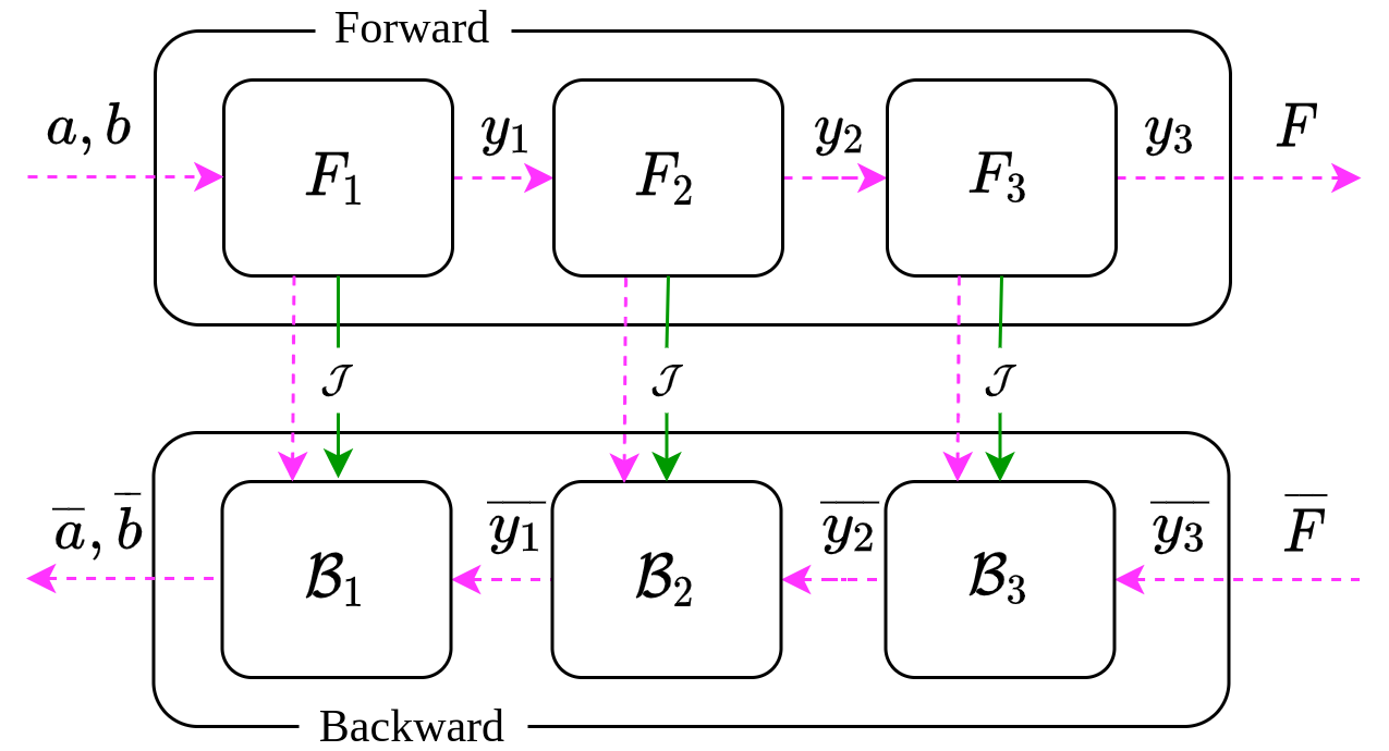
We will now see how gradients of a complex function (given its full specification) can be computed as a sequence of primitive operations. Let’s explain this with an example for simplicity: We have two inputs \(a, b\) (just symbols) and a description of the scalar function we want to differentiate:
\[ \displaystyle{F(a, b) = \frac{a}{1+b^2}} \]
We can think of \(F(a, b)\) as a series of smaller computations with intermediate results, like this
\[ \begin{align} y_1 &← pow(b, 2) \\ y_2 &← add(1, y_1) \\ y_3 &← div(a, y_2) \end{align} \]
I changed the pure math notations to more programmatic ones; but the meaning remains same. In order to compute gradients, we augment these computations and create something called a “pullback” function as an additional by-product.
Mathematically, the actual computation and pullback creation can be written together symbolically as:
\[ \tag{1} \begin{align} y_1, \mathcal{B}_1 &← \mathcal{J}(pow, b, 2) \\ y_2, \mathcal{B}_2 &← \mathcal{J}(add, 1, y_1) \\ y_3, \mathcal{B}_3 &← \mathcal{J}(div, a, y_2) \end{align} \]
You can think of the functional \(\mathcal{J}\) as the internals of the Backpropagation framework which mutates all the computation units to produce an extra entity. A pullback function (\(\mathcal{B}_i\)) is a function that takes input the gradient w.r.t the output of the corresponding function and returns the gradient w.r.t inputs of the function:
\[ \mathcal{B}_i : \overline{y}_i \rightarrow \overline{input_1}, \overline{input_2}, \cdots \]
It is really nothing but a different view of the chain-rule of differentiation:
\[ \begin{align} \frac{\partial F}{\partial b} &\leftarrow \mathcal{B}_1(\frac{\partial F}{\partial y_1}) \triangleq \frac{\partial F}{\partial y_1} \cdot \frac{\partial y_1}{\partial b} \\ \overline{b} &\leftarrow \mathcal{B}_1( \overline{y}_1 ) \triangleq \overline{y}_1 \cdot \frac{\partial y_1}{\partial b}\left[ \text{Denoting } \frac{\partial F}{\partial x}\text{ as }\overline{x} \right] \end{align} \]
We must also realize that computing \(\mathcal{B}_i\) may require values from the forward pass. For example, computing \(\overline{b}\) may need evaluating \(\displaystyle{ \frac{\partial y_1}{\partial b} }\) at the given value of \(b\). After getting access to \(\mathcal{B}_i\), we can compute the derivatives of \(F\) w.r.t \(a, b\) by invoking the pullback functions in proper (reverse) order
\[ \begin{align} \overline{a}, \overline{y_2} &\leftarrow \mathcal{B}_3(\overline{y}_3) \\ \overline{y_1} &\leftarrow \mathcal{B}_2(\overline{y}_2) \\ \overline{b} &\leftarrow \mathcal{B}_1(\overline{y}_1) \end{align} \]
Please note that \(y_3\) is actually \(F\) and hence \(\overline{y}_3 ≜ \displaystyle{ \frac{\partial F}{\partial y_3} = 1 }\).
1. Tape-based implementation
There are couple of different ways of implementing the theory described above. The de-facto way of doing it (as of this day) is something known as “tape-based” implementation. PyTorch and Tensorflow Eager Execution are probably the most popular example of this type.
In tape-based systems, the function \(F(..)\) is specified by its full structural form. Moreover, it requires runtime execution in order to compute anything (be it output or derivatives). Such system keeps track of every computation via a recorder or “tape” (that’s why the name) and builds an internal computation graph. Later, when requested, the tape stops recording and works its way backwards through the recorded tape to compute derivatives.
The specification of \(F(\Theta)\)
A tape-based system requires users to provide the function \(F\) as a description of its computations following a certain guidelines. These guidelines are provided by the specific AutoDiff framework we use. Take PyTorch for example - we write the series of computations using the API provided by PyTorch:
import torch

class Network(torch.nn.Module):
    def __init__(self):
        self.b0 = ...

    def forward(self, a):
        y1 = torch.pow(self.b0, 2)
        y2 = torch.sum(1, y1)
        y3 = torch.div(a, y2)
        return y3
Think of the framework as an entity which is solely responsible for doing all the derivative computations. You just can’t be careless to use math.sum() (or anything) instead torch.sum(), or omit the base class torch.nn.Module. You have to stick to the guidelines PyTorch laid out to be able to make use of it. When done with the definition, we can run forward and backward pass like using actual data \((a_0, b_0)\)
model = Network(...)
F = model(a0)
F.backward()
# 'model.b0.grad' & 'a0.grad' available
This will cause the framework to trigger the following sequence of computations one after another
\[ \tag{2} \begin{align} y_1, \mathcal{B}_1 &← \mathcal{J}(\mathrm{torch.pow}, \mathbf{b_0}, 2) \\ y_2, \mathcal{B}_2 &← \mathcal{J}(\mathrm{torch.sum}, 1, y_1) \\ y_3, \mathcal{B}_3 &← \mathcal{J}(\mathrm{torch.div}, \mathbf{a_0}, y_2) \\ \left[ \overline{a}\right]_{a=\mathbf{a_0}}, \overline{y_2} &\leftarrow \mathcal{B}_3(1) \\ \overline{y_1} &\leftarrow \mathcal{B}_2(\overline{y}_2) \\ \left[ \overline{b}\right]_{b=\mathbf{b_0}} &\leftarrow \mathcal{B}_1(\overline{y}_1) \end{align} \]
The first and last 3 lines of computation are the “forward pass” and the “backward pass” of the model respectively. Frameworks like PyTorch and Tensorflow typically works in this way when .forward() and .backward() calls are made in succession. Point to be noted that since we are explicitly executing a forward pass, it will cache the necessary values required for executing the pullbacks in the backward pass. An overall diagram is shown below for clarification.
What’s the problem ?
As of now, it might not seem that big of a problem for regular PyTorch user (me included). The problem intensifies when you have a non-ML code base with a complicated physics model (for example) like this
import math
from other_part_of_my_model import sub_part

def helper_function(x):
    if something:
        return helper_function(sub_part(x-1)) # recursive call
    ...

def complex_physics_model(parameters, input):
    math.do_awesome_thing(parameters, helper_function(input))
    ...
    return output
.. and you want to use it within your PyTorch model and differentiate it. There is no way you can do this so easily without spending your time to PyTorch-ify it first.
There is another serious problem with this approach: the framework cannot “see” any computation ahead of time. For example, when the execution thread reaches the torch.sum() function, it has no idea that it is about to encounter torch.div(). The reason its important is because the framework has no way of optimizing the computation - it has to execute the exact sequence of computations verbatim. For example, if the function description is given as \(\displaystyle{ F(a, b) = \frac{(a + ab)}{(1 + b)} }\), this type of framework will waste its resources executing lots of operations which will ultimately yield (both in forward and backward direction) something trivial.
2. Differentiable Programming
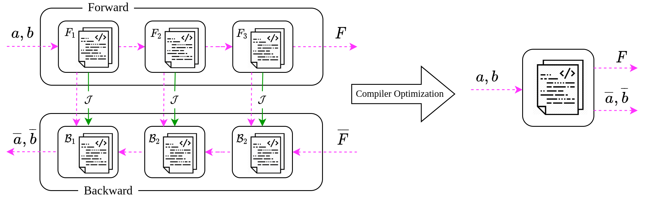
Differentiable Programming (DiffProg) offers a very elegant solution to both the problems described in the previous section. DiffProg allows you to write arbitrary code without following any guidelines and still be able to differentiate it. At the current state of DiffProg, majority of the successful systems use something called “source code transformation” in order to achieve its objective.
Source code transformation is a technique used extensively in the field of Compiler Designing. It takes a piece of code written in some high-level language (like C++, Python etc.) and emits a compiled version of it typically in a relatively lower level language (like Assembly, Bytecode, IRs etc.). Specifically, the input to a DiffProg system is a description of \(y ← F(\Theta)\) as source code written in some language with defined input/output. The output of the system is the source code of the derivative of \(F(\Theta)\) w.r.t its inputs (i.e., \(\overline{\Theta} ← F'(\overline{y})\)). The input program has full liberty to use the native primitives of the programming language like built-in functions, conditional statements, recursion, struct-like facilities, memory read/write constructs and pretty much anything that the language offers.
Using our generic notation, we can write down such a system as
\[ y, \mathcal{B} \leftarrow \mathcal{J}(F, \Theta) \]
where \(F\) and \(\mathcal{B}:\overline{y}\rightarrow \overline{\Theta}\) are the given function and its derivative function in the form of source codes (bare with me if it doesn’t make sense at this point). Just like before, the source code for pullback \(\mathcal{B}\) may require some intermediate variables from that of \(y\). For a concrete example, the following is be a (hypothetical) valid DiffProg system:
>>> # following string contains the source code of F(.)
>>> input_prog = """
def F(a, b):
    y1 = b ** 2
    y2 = 1 + y1
    return a / y2
"""
>>> y, B = diff_prog(input_prog, a=1., b=2.)
>>> print(y)
0.2
>>> exec(B) # get the derivative function as a live object in current session
>>> print(dF(1.)) # 'df()' is defined in source code 'B'
(0.2, -0.16)
Please pay attention to the fact that both our problems discussed in tape-based system are effectively solved now:
We no longer need to be under the umbrella of a framework as we can directly work with native code. In the above example, the source code of the given function is simply written in native python. The example shows the overall pullback source-code (i.e.,
B) and also its explicitly compiled form (i.e.,dF). Optionally, a DiffProg system can produce readily compiled derivative function.The DiffProg system can “see” the whole source-code at once, giving it the opportunity to run various optimizations. As a result, both the given program the derivative program could be much faster than the standard tape-based approaches.
Although I showed the examples in Python for ease of understanding but it doesn’t really have to be Python. The theory of DiffProg is very general and can be adopted to any language. In fact, Python is NOT the language of choice for some of the first successful DiffProg systems. The one we are gonna talk about is written in a relatively new language called Julia. The Julia language and its compiler provides an excellent support for meta-programming, i.e. manipulating/analysing/constructing Julia programs within itself. This allows Julia to offer a DiffProg system that is much more flexible than naively parsing strings (like the toy example shown above). We will look into the specifics of the Julia language and its DiffProg framework called “Zygote” later in this article. But before that, we will look at few details about the general compiler machinery that is required to implement DiffProg systems. Since this article is mostly targetted towards people from ML/DL background, I will try my best to be reasonable about the details of compiler designing.
Static Single Assignment (SSA) form
A compiler (or compiler-like system) analyses a given source code by parsing it as string. Then, it creates a large and complex data structure (known as AST) containing control flow, conditionals and every fundamental language constructs. Such structure is further compiled down to a relatively low-level representation comprising the core flow of a source program. This low-level code is known as the “Intermediate Representation (IR)”. One of its fundamental purpose is to replaces all unique variable names with a unique ID. A given source code like this
function F(a, b)
    y1 = b ^ 2
    y1 = 1 + y1
    return a / y1
a compiler can turn it into an IR (hypothetical) like
function F(%1, %2)
    %3 = %2 ^ 2
    %3 = 1 + %3
    return %1 / %3
where %N is a unique placeholder for a variable. However, this particular form is a little inconvenient to analyse in practice due to the possibility of a symbol redefinition (e.g. the variable y1 in above example). Modern compilers (including Julia) use a little improved IR, called “SSA (Static Single Assignment) form IR” which assigns one variable only once and often introduces extra unique symbols in order to achieve that.
function F(%1, %2)
    %3 = %2 ^ 2
    %4 = 1 + %3
    return %1 / %4
Please note how it used an extra unique ID (i.e. %4) in order to avoid re-assignment (of %3). It has been shown that such SSA-form IR (rather than direct source code) can be differentiated, and a corresponding “Derivative IR” can be retrieved. The obvious way of crafting the derivative IR of \(F\) is to use the Derivative IRs of its constituent operations, similar to what is done in tape-based method. The biggest difference is the fact that everything is now in terms of source codes (or rather IR to be precise). The compiler could craft the derivative program like this
function dF(%1, %2)
    # IR for forward pass
    %3, B1 = J(pow, %2, 2)
    %4, B2 = J(add, 1, %3)
    _, B3 = J(div, %1, %4)

    # IR for backward pass
    %5, %6 = B3(1)
    %7 = B2(%6)
    %8 = B1(%7)
    return %5, %8
The structure of the above code may resemble the sequence of computations in Eq.2, but its very different in terms of implementation (Refer to Fig.2 below). The code (IR) is constructed at compile time by a compiler-like framework (the DiffProg system). The derivative IR is then passed onto an IR-optimizer which can squeeze its guts by enabling various optimization like dead-code elimination, operation-fusion and more advanced ones. And finally compiling it down to machine code.
Zygote: A DiffProg framework for Julia
Julia is a particularly interesting language when it comes to implementing a DiffProg framework. There are solid reasons why Zygote, one of the most successful DiffProg frameworks is written in Julia. I will try to articulate few of them below:
Just-In-Time (JIT) compiler: Julia’s efficient Just-in-time (JIT) compiler compiles one statement at a time and run it immediately before moving on to the next one, achieving a striking balance between interpreted and compiled languages.
Type specialization: Julia allows writing generic/optional/loosely-typed functions that can later be instantiated using concrete types. High-density computations specifically benefit from it by casting every computation in terms of
Float32/Float64which can in turn produce specialized instructions (e.g.AVX,MMX,AVX2) for modern CPUs.Pre-compilation: The peculiar feature that benefits
Zygotethe most is Julia’s nature of keeping track of the compilations that have already been done in the current session and DOES NOT do them again. Since DL/ML is all about computing gradients over and over again,Zygotecompiles and optimizes the derivative program (IR) just once and runs it repeatedly (which is blazingly fast) with different value of parameters.LLVM IR: Julia uses LLVM compiler infrastructure as its backend and hence emits the LLVM IR known to be highly performant and used by many other prominent languages.
Now, let’s see Zygote’s primary API, which is surprisingly simple. The central API of Zygote is the function Zygote.gradient(..) with its first argument being the function to be differentiated (written in native Julia) followed by its argument at which gradient to be computed.
julia> using Zygote
julia> function F(x)
           return 3x^2 + 2x + 1
       end
julia> gradient(F, 5)
(32,)
That is basically computing \(\displaystyle{ \left[ \frac{\partial F}{\partial x} \right]_{x=5} }\) for \(F(x) = 3x^2 + 2x + 1\).
For debugging purpose, we can see the actual LLVM IR code for a given function and its pullback. The actual IR is a bit more complex in reality than what I showed but similar in high-level structure. We can peek into the IR of the above function
julia> Zygote.@code_ir F(5)
1: (%1, %2)
  %3 = Core.apply_type(Base.Val, 2)
  %4 = (%3)()
  %5 = Base.literal_pow(Main.:^, %2, %4)
  %6 = 3 * %5
  %7 = 2 * %2
  %8 = %6 + %7 + 1
  return %8
.. and also its “Adjoint”. The adjoint in Zygote is basically the mathematical functional \(\mathcal{J}(\cdot)\) that we’ve been seeing all along.
julia> Zygote.@code_adjoint F(5)
Zygote.Adjoint(1: (%3, %4 :: Zygote.Context, %1, %2)
  %5 = Core.apply_type(Base.Val, 2)
  %6 = Zygote._pullback(%4, %5)
  ...
  # please run yourself to see the full code
  ...
  %13 = Zygote.gradindex(%12, 1)
  %14 = Zygote.accum(%6, %10)
  %15 = Zygote.tuple(nothing, %14)
  return %15)
I have established throughout this article that the function \(F(x)\) can literally be any arbitrary program written in native Julia using standard language features. Let’s see another toy (but meaningful) program using more flexible Julia code.
struct Point
    x::Float64
    y::Float64
    Point(x::Real, y::Real) = new(convert(Float64, x), convert(Float64, y))
end

# Define operator overloads for '+', '*', etc.

function distance(p₁::Point, p₂::Point)::Float64
    δp = p₁ - p₂
    norm([δp.x, δp.y])
end

p₁, p₂ = Point(2, 3.0), Point(-2., 0)
p = Point(-1//3, 1.0)

# initial parameters
K₁, K₂ = 0.1, 0.1
for i = 1:1000 # no. of epochs

    # compute gradients
    @time δK₁, δK₂ = Zygote.gradient(K₁, K₂) do k₁::Float64, k₂::Float64
        p̂ = p₁ * k₁ + p₂ * k₂
        distance(p̂, p) # scalar output of the function
    end

    # update parameters
    K₁ -= 1e-3 * δK₁
    K₂ -= 1e-3 * δK₂
end
@show K₁, K₂
# shows "(K₁, K₂) = (0.33427804653861276, 0.4996408206795386)"
The above program is basically solving the following (pretty simple) problem
\[ \begin{align} \arg\min_{K_1,K_2} &\vert\vert \widehat{p}(K_1,K_2) - p \vert\vert_2 \\ \text{with }&\widehat{p}(K_1,K_2) ≜ p_1 \cdot K_1 + p_2 \cdot K_2 \end{align} \]
where \(p=[-1/3, 1]^T, p_1=[2,3]^T\) and \(p_2=[-2,0]^T\). By choosing these specific numbers, I guaranteed that there is a solution for \(K_1,K_2\).
If you look at the program at a glance, you would notice that the whole program is almost entirely written in native Julia using structure (struct Point), built-in function (norm(), convert()), memory access constructs (δp.x, δp.y) etc. The only usage of Zygote is that Zygote.gradient() call in the heart of the loop. BTW, I omitted the operator overloading functions for space restrictions.
I am not showing the IR codes for this one; you are free to execute @code_ir and @code_adjoint on the function implicitly defined using the do .. end. One thing I would like to show is the execution speed and my earlier argument about “precompilation”. The time measuring macro (@time) shows this
 11.764279 seconds (26.50 M allocations: 1.342 GiB, 4.58% gc time)
  0.000025 seconds (44 allocations: 2.062 KiB)
  0.000026 seconds (44 allocations: 2.062 KiB)
  0.000007 seconds (44 allocations: 2.062 KiB)
  0.000006 seconds (44 allocations: 2.062 KiB)
  0.000005 seconds (44 allocations: 2.062 KiB)
  0.000005 seconds (44 allocations: 2.062 KiB)
Did you see how the execution time reduced by an astonishingly high margin ? That’s Julia’s precompilation at work - it compiled the derivative program only once (on its first encounter) and produces highly efficient code to be reused later. It might not be as big a surprise if you already know Julia, but it is definitely a huge advantage for a DiffProg framework.
Okay, that’s about it today. See you next time. The following references have been used for preparing this article:
- “Don’t Unroll Adjoint: Differentiating SSA-Form Programs”, Michael Innes, arXiv/1810.07951.
- Talk by Michael Innes @ Julia london user group meetup.
- Talk by Elliot Saba & Viral Shah @ Microsoft research.
- Zygote’s documentation & Julia’s documentation.
Citation
@online{das2020,
  author = {Das, Ayan},
  title = {Differentiable {Programming:} {Computing} Source-Code
    Derivatives},
  date = {2020-09-08},
  url = {https://ayandas.me/blogs/2020-09-08-differentiable-programming.html},
  langid = {en}
}