Foundation of Variational Autoencoder (VAE)

In the previous article, I started with Directed Probabilitic Graphical Models (PGMs) and a family of algorithms to do efficient approximate inference on them. Inference problems in Directed PGMs with continuous latent variables are intractable in general and require special attention. The family of algorithms, namely Variation Inference (VI), introduced in the last article is a general formulation of approximating the intractable posterior in such models. Variational Autoencoder or famously known as VAE is an algorithm based on the principles on VI and have gained a lots of attention in past few years for being extremely efficient. With few more approximations/assumptions, VAE eshtablished a clean mathematical formulation which have later been extended by researchers and used in numerous applications. In this article, I will explain the intuition as well as mathematical formulation of Variational Autoencoders.

Variational Inference: A recap

A quick recap would make going forward easier.

Given a Directed PGM with countinuos latent variable $Z$ and observed variable $X$, the inference problem for $Z$ turned out to be intractable because of the form of its posterior

$$\mathbb{P}(Z|X)=\frac{\mathbb{P}(X,Z)}{\mathbb{P}(X)}=\frac{\mathbb{P}(X,Z)}{\sum _Z\mathbb{P}(X,Z)}$$

To solve this problem, VI defines a parameterized approximation of $\mathbb{P}(Z|X)$, i.e., $\mathbb{Q}(Z;\varphi )$ and formulates it as an optimization problem

$${\mathbb{Q}}^{\ast }(Z)=arg\underset{\varphi }{min}\mathbb{K}\mathbb{L}[\mathbb{Q}(Z;\varphi )||\mathbb{P}(Z|X)]$$

The objective can further be simplified as

$$\mathbb{K}\mathbb{L}[\mathbb{Q}(Z;\varphi )||\mathbb{P}(Z|X)]$$ $$={\mathbb{E}}_{\mathbb{Q}}[\log \mathbb{Q}(Z;\varphi )]-{\mathbb{E}}_{\mathbb{Q}}[\log \mathbb{P}(X,Z)]\triangleq -ELBO(\mathbb{Q})$$

$ELBO(\mathbb{Q})$ is precisely the objective we maximize. The $ELBO(\cdot )$ can best be explained by decomposing it into two factors. One of them takes care of maximizing the expected conditional log-likelihood (of the data given latent) and the other arranges the latent space in a way that it matches a predifined distribution.

$$ELBO(\mathbb{Q})={\mathbb{E}}_{\mathbb{Q}}[\log \mathbb{P}(X|Z)]-\mathbb{K}\mathbb{L}[\mathbb{Q}(Z;\varphi )||\mathbb{P}(Z)]$$

For a detailed explanation, go through the previous article.

Variational Autoencoder

Variational Autoencoder (VAE) is first proposed in the paper titled “Auto-Encoding Variational Bayes” by D.P.Kingma & Max Welling. The paper proposes two things:

1. A parameterized inference model instead of just $\mathbb{Q}(Z;\varphi )$
2. The reparameterization trick to achieve efficient training

As we go along, I will try to convey the fact that these are essentially developments on top of the general VI framework we learnt earlier. I will focus on how each of them is related to VI in the following (sub)sections.

The “Inference Model”

Fig.1. Subfig.1: The Bayesian Network defining VAE. Subfig.2: The forward pass (abstarct) of VAE. Subfig.3: The forward pass of VAE with explicit sampling shown at the end of encoder

The idea is to replace the generically parameterized $\mathbb{Q}(Z;\varphi )$ in the VI framework by a data-driven model $\mathbb{Q}(Z|X;\varphi )$, named as Inference model. What does it mean ? It basically means, we are no longer interested in the unconditional distribution on $Z$ but instead we want to have a conditional distribution on $Z$ given observed data. Please recall our “generative view” of the model

$$z^{(i)}\sim \mathbb{P}(Z)$$ $$x^{(i)}\sim \mathbb{P}(X|Z=z^{(i)})$$

With the inference model in hand, we now have an “inference view” as follows

$$z^{(i)}\sim \mathbb{P}(Z|X=x^{(i)})$$

It means, we can do inference just by ancestral sampling after our model is trained. Of course, we don’t know the real $\mathbb{P}(Z|X)$, so we consider a parameterized approximation $\mathbb{Q}(Z|X;\varphi )$ as I already mentioned.

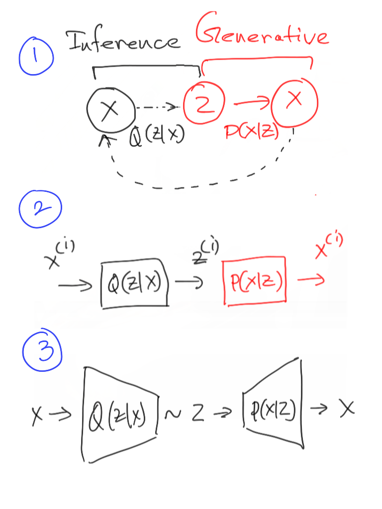
These two “views”, when combined, forms the basis of Variational Autoencoder (See Fig.1: Subfig.1).

$$z^{(i)}\sim \mathbb{P}(Z|X=x^{(i)})$$ $$x^{(i)}\sim \mathbb{P}(X|Z=z^{(i)})$$

The “combined model” shown above gives us insight about the training process. Please note that the model starts from $x^{(i)}$ (a data sample from our dataset) - generates $z^{(i)}$ via the Inference model - and then maps it back to $x^{(i)}$ again using the Generative model (See Fig.1: Subfig.2). I hope the reader can now guess why its called an Autoencoder ! So, we clearly have a computational advantage here: we can perform training on per-sample basis; just like Inference. This is not true for many of the approximate inference algorithms of pre-VAE era.

So, succinctly, all we have to do is a “forward pass” through the model (yes, the two sampling equations above) and maximize $\log \mathbb{P}(X=x^{(i)}|Z=z^{(i)};\theta )$ where $z^{(i)}$ is a sample we got from the Inference model. Note that we need to parameterize the generative model as well (with $\theta$). In general, we almost always choose $\mathbb{Q}(\cdot ;\varphi )$ and $\mathbb{P}(\cdot ;\theta )$ as a fully-differentiable functions like Neural Network (See Fig.1: Subfig.3 for a cleaner diagram). Now we go back to our objective function from VI framework. To formalize the training objective for VAE, we just need to replace $\mathbb{Q}(Z;\varphi )$ by $\mathbb{Q}(Z|X;\varphi )$ in the VI framework (please compare the equations with the recap section)

$${\mathbb{Q}}^{\ast }(Z|X)=arg\underset{\varphi }{min}\mathbb{K}\mathbb{L}[\mathbb{Q}(Z|X;\varphi )||\mathbb{P}(Z|X)]$$

And the objective

$$\mathbb{K}\mathbb{L}[\mathbb{Q}(Z|X;\varphi )||\mathbb{P}(Z|X)]$$ $$={\mathbb{E}}_{\mathbb{Q}}[\log \mathbb{Q}(Z|X;\varphi )]-{\mathbb{E}}_{\mathbb{Q}}[\log \mathbb{P}(X,Z)]\triangleq -ELBO(\mathbb{Q})$$

Then,

$$ELBO(\mathbb{Q})={\mathbb{E}}_{\mathbb{Q}}[\log \mathbb{P}(X|Z;\theta )]-\mathbb{K}\mathbb{L}[\mathbb{Q}(Z|X;\varphi )||\mathbb{P}(Z)]$$

As usual, $\mathbb{P}(Z)$ is a chosen distribution which we want the structure of $\mathbb{Q}(Z|X;\varphi )$ to be; which is often Standard Gaussian/Normal (i.e., $\mathbb{P}(Z)=\mathcal{N}(0,I)$)

$$\mathbb{Q}(Z|X;[{\varphi }_1,{\varphi }_2])=\mathcal{N}(Z;\mu (X;{\varphi }_1),\sigma (X;{\varphi }_2))$$

The specific parameterization of $\mathbb{Q}(Z|X;[{\varphi }_1,{\varphi }_2])$ reveals that we predict a distribution in the forward pass just by predicting its parameters.

The first term of $ELBO(\cdot )$ is relatively easy, its a loss function that we have used a lot in machine learning - the log-likelihood. Very often it is just the MSE loss between the predicted $\hat{X}$ and original data $X$. What about the second term ? It turns out that we can have closed-form solution for that. Because I don’t want unnecessary maths to clutter this post, I am just putting the formula for the readers to look at. But, I would highly recommend looking at the proof in Appendix B of the original VAE paper. Its not hard, believe me. So, putting the proper values of $\mathbb{Q}(Z|\cdot )$ and $\mathbb{P}(Z)$ into the KL term, we get

$$\mathbb{K}\mathbb{L}[\mathcal{N}(\mu (X;{\varphi }_1),\sigma (X;{\varphi }_2))||\mathcal{N}(0,I)]$$

$$=\frac{1}{2}\sum _j(1+\log {\sigma }_j^2-{\mu }_j^2-{\sigma }_j^2)$$

Please note that ${\mu }_j,{\sigma }_j$ are the individual dimensions of the predicted mean and std vector. We can easily compute this in forward pass and add it to the log-likelihood (first term) to get the full (ELBO) loss.

Okay. Let’s talk about the forward pass in a bit more detail. Believe me, its not as easy as it looks. You may have noticed (Fig.1: Subfig.3) that the forward pass contains a sampling operation (sampling $z^{(i)}$ from $\mathbb{P}(Z|X=x^{(i)})$) which is NOT differentiable. What do we do now ?

The reparameterization trick

Fig.1. Subfig.1: The full forward pass. Subfig.2: The full forward pass with reparameterized sampling.

I showed before that in forward pass, we get the $z^{(i)}$ by sampling from our parameterized inference model. Now that we know the exact form of the inference model, the sampling will look something like this

$$z^{(i)}\sim \mathcal{N}(Z|\mu (X;{\varphi }_1),\sigma (X;{\varphi }_2))$$

The idea is basically to make this sampling operation differentiable w.r.t $\mu$ and $\sigma$. In order to do this, we pull a trick like this

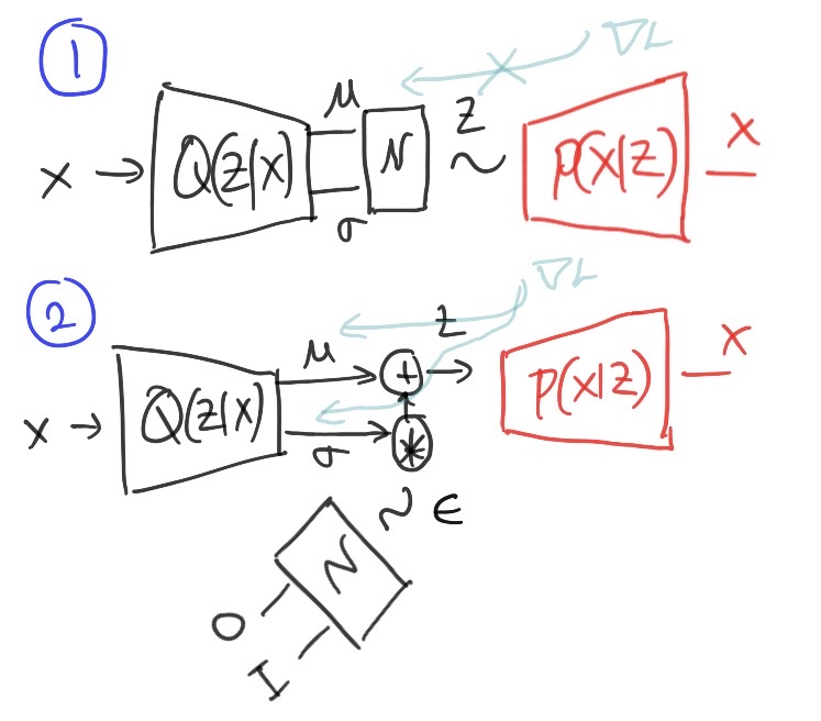
$$z^{(i)}={\mu }^{(i)}+{ϵ}^{(i)}\ast {\sigma }^{(i)}\text{ , where }{ϵ}^{(i)}\sim \mathcal{N}(0,I)$$

This is known as the “reparameterization”. We basically rewrite the sampling operation in a way that separates the source of randomness (i.e., ${ϵ}^{(i)}$) from the deterministic quantities (i.e., $\mu$ and $\sigma$). This allows the backpropagation algorithm to flow derivatives into $\mu$ and $\sigma$. However, please note that it is still not differentiable w.r.t $ϵ$ but .. guess what .. we don’t need it ! Just having derivatives w.r.t $\mu$ and $\sigma$ is enough to flow it backwards and pass it to the parameters of inference model (i.e., $\varphi$). Fig.2 should make everything clear if not already.

---

Wrap up

That’s pretty much it. To wrap up, here is the full forward-backward algorithm for training VAE:

1. Given $x^{(i)}$ from the dataset, compute $\mu (x^{(i)},{\varphi }_1),\sigma (x^{(i)},{\varphi }_1)$.
2. Compute a latent sample as $z^{(i)}={\mu }^{(i)}+{ϵ}^{(i)}\ast {\sigma }^{(i)}\text{ , where }{ϵ}^{(i)}\sim \mathcal{N}(0,I)$
3. Compute the full loss as $L=\log \mathbb{P}(x^{(i)}|Z=z^{(i)})+\frac{1}{2}\sum _j(1+\log {\sigma }_j^2-{\mu }_j^2-{\sigma }_j^2)$.
4. Update parameters as $\{\varphi ,\theta \}:=\{\varphi ,\theta \}-\eta \frac{\delta L}{\delta \{\varphi ,\theta \}}$
5. Repeat.