Welcome folks ! This is an article I was planning to write for a long time. I finally managed to get it done while locked at home due to the global COVID-19 situation. So, its basically something fun, interesting, attractive and hopefully understandable to most readers. To be specific, my plan is to dive into the world of finding visually appealing patterns in different sections of mathematics. I am gonna introduce you to four distinct mathematical concepts by means of which we can generate artistic patterns that are very soothing to human eyes. Most of these use random number as the underlying principle of generation. These are not necessarily very useful in real life problem solving but widely loved by artists as a tool for content creation. They are sometimes referred to as Mathematical Art. I will deliberately keep the fine-grained details out of the way so that it is reachable to a larger audience. In case you want to reproduce the content in this post, here is the code. Warning: This post contains quite heavily sized images which may take some time to load in your browser; so be patient.
Random Walk & Brownian Motion
Let’s start with something simple. Consider a Random Variable \(\mathbf{R}_t\) (\(t\) being time) with support \(\{ -1, +1\}\) with equal probability on both of its possible values. Think of it as a score you get at time \(t\) which can be either \(+1\) or \(-1\) as a result of an unbiased coin-flip. In terms of probability:
\[ \mathbb{P}\bigl[ \mathbf{R}_t = +1 \bigr] = \mathbb{P}\bigl[ \mathbf{R}_t = -1 \bigr] = \frac{1}{2} \]
Realization (samples) of \(\mathbf{R}_t\) for \(t=0 \rightarrow T (=10)\) would look like \[ \bigl[ +1, -1, -1, +1, -1, -1, -1, +1, +1, -1, +1 \bigr] \]
Let us define another Random Variable \(\mathbf{S}_t\) which is nothing but an accumulator of \(\mathbf{R}_t\) till time \(t\). So, by definition
\[ \mathbf{S}\_t = \sum_{i=0}^t \mathbf{R}\_i \] Realization of \(\mathbf{S}_t\) corresponding to above \(\mathbf{R}_t\) sequence would look like \[ \bigl[ +1, 0, -1, 0, -1, -2, -3, -2, -1, -2, -1 \bigr] \]
This is popularly known as the Random Walk. With the basics ready, let us have two such random walks namely \(\mathbf{S}^x_t\) and \(\mathbf{S}^y_t\) and treat them as \(X\) and \(Y\) coordinates of a Random Vector namely \(\displaystyle{ \bar{\mathbf{S}}_t \triangleq \begin{bmatrix} \mathbf{S}^x_t \\ \mathbf{S}^y_t \end{bmatrix} }\).
As of now it look all nice and mathy, right ! Here’s the fun part. Let me keep the time (i.e., \(t\)) running and keep track on the path that the vector \(\bar{\mathbf{S}}_t\) traces on a 2D plane
It will create a cool random checkerboard-like pattern as time goes on. Looking at the tip (the ‘dot’), you might see it as a tiny particle. As it happened that this is a discretized verision of a continuous phenomenon observed in real microscopic particles in fluid, famously known as Brownian Motion.
Real Brownian Motion is continuous. Let’s work it out, but very briefly. We divide an arbitrary time interval \([0, T]\) into \(N\) small intervals of length \(\displaystyle{ \Delta t = \frac{T}{N} }\) and have a modified score Random Variable \(\mathbf{R}_t\) with support \(\displaystyle{ \left\{ +\sqrt{\frac{T}{N}}, -\sqrt{\frac{T}{N}} \right\} }\) with equal probability as before. We still have the same definition of \(\mathbf{S}_t = \sum_{i=0}^t \mathbf{R}_i\). It so happened that as we appraoch the limiting case of
\[ N \rightarrow \infty,\text{ and consequently } \sqrt{\frac{T}{N}} \rightarrow 0\text{ and } \Delta t\rightarrow 0 \]
it gives us the continuous analogue of Brownian Motion. Similar to the discrete case, if we trace the path of \(\displaystyle{ \bar{\mathbf{S}}_t \triangleq \begin{bmatrix} \mathbf{S}^x_t \\ \mathbf{S}^y_t \end{bmatrix} }\) with large \(N\) (yes, in practice we cannot go to infinity, sorry), patterns like this will emerge
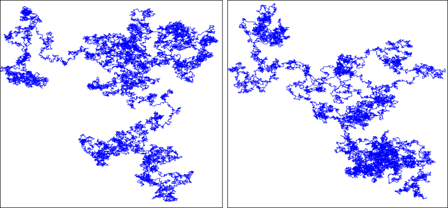
To make it more artistic, I took an even bigger \(N\) and ran the simulation for quite a while and got quite beautiful jittery patterns. Random numbers being at the heart of the phenomenon, we’ll get different patterns in different runs. Here are two such simulation results:
Want to learn more ?
Dynamical Systems & Chaos
Dynamical Systems are defined by a state space \(\mathbb{R}^n\) and a system dynamics (a function \(\mathbf{F}\)). A state \(\mathbf{x}\in\mathbb{R}^n\) is a specific (abstract) configuration of a system and the dynamics determines how the state “evolves” over time. The dynamics is often represented by a differential equation that specifies the chnage of state over time. So,
\[ \mathbf{F}(\mathbf{x}, t) \triangleq \frac{d\mathbf{x}}{dt} \]
The true states of the system at some point of time is determined by solving and Initial Value Problem (IVP) starting from an initial state \(\mathbf{x}_0\). We then solve consecutive states with \(t\gt 0\) as
\[ \mathbf{x}_t = \mathbf{x}_0 + \Delta t \cdot \mathbf{F}(\mathbf{x}, t) \]
Having sufficiently small \(\Delta t\) ensures propert evolution of states.
Now this may seem quite trivial, at least to those who have studied Differential Equations. But, there are specific cases of \(\mathbf{F}\) which leads to an evolution of states whose trajectory is surprisingly beautiful. For reasons that are beyond the scope of this article, these are called Chaos. There is a specific branch of dynamical systems (named “Chaos Theory”) that deals with characteristics of such chaotic systems. Below are three such chaotic systems with there trajectory visualized in 3D state space. To be specific, we take each system with an initial state (they are very sensitive to initial states) and compute successive states with a small enough \(\Delta t\) and visualize them as a continuous path in 3D. The corresponding figures depict an animation of the evolution of states over time as well as the whole trajectory all at once.
Lorentz System
\[ \frac{d\mathbf{x}}{dt} = \bigl[ \sigma (y-x), x(\rho - z) - y, xy - \beta z \bigr]^T \] \[ \text{with }\sigma = 10, \beta = \frac{8}{3}, \rho = 28 \text{, and } \mathbf{x}_0 = \bigl[ 1,1,1 \bigr] \]
Rössler System
\[ \frac{d\mathbf{x}}{dt} = \bigl[ -(y+z), x+Ay, B+xz-Cz \bigr]^T \] \[ \text{with }A=0.2, B=0.2, C=5.7 \text{, and } \mathbf{x}_0 = \bigl[ 1,1,1 \bigr] \]
Halvorsen System
\[ \frac{d\mathbf{x}}{dt} = \bigl[ -ax-4y-4z-y^2, -ay-4z-4x-z^2, -az-4x-4y-x^2 \bigr]^T \] \[ \text{with }a=1.89 \text{, and } \mathbf{x}_0 = \bigl[ -1.48, -1.51, 2.04 \bigr] \]
Want to learn more ?
Complex Fourier Series
We all know about Fourier Series, right ! But I am sure not all of you have seen this artistic side of it. Well, this isn’t really related to fourier series, but fourier series helps in creating them.
We know the following to be the “synthesis equation” of complex fourier series
\[ f(t) = \sum_{n=-\infty}^{+\infty} c_n e^{j \frac{2\pi n}{T} t} \in \mathbb{C} \]
which represents the synthesis of a periodic function \(f(t)\) of period \(T\) from its frequency components \(\mathbf{C} \triangleq \left[ c_{-\infty}, \cdots, c_{-2}, c_{-1}, c_{0}, c_{+1}, c_{+2}, \cdots, c_{+\infty} \right]\). Often, as a practical measure, we crop the infinite summation to a limited range \([ -N, N ]\). Furthermore, let’s consider \(T=1\) without lose of generality. So, we see \(f(t)\) as a function parameterized by the frequence components \(\mathbf{C} \in \mathbb{C}^{2N+1}\)
\[ f(t, \mathbf{C}) \approx \sum_{n=-N}^{+N} c_n e^{j 2\pi n t} \in \mathbb{C} \]
By doing this, we can make complex valued functions by putting different \(\mathbf{C}\) and running \(t=0\rightarrow 1\). However, not all \(\mathbf{C}\) leads to anything visually appealing. A particular feature of an object that appeals to the human eyes is “Symmetry”. We are gonna exploit this here. A little refresher on fourier series will make you realize that if the coefficients are real-valued, then \(f(t, \mathbf{C})\) has symmetric property. And that’s all we need.
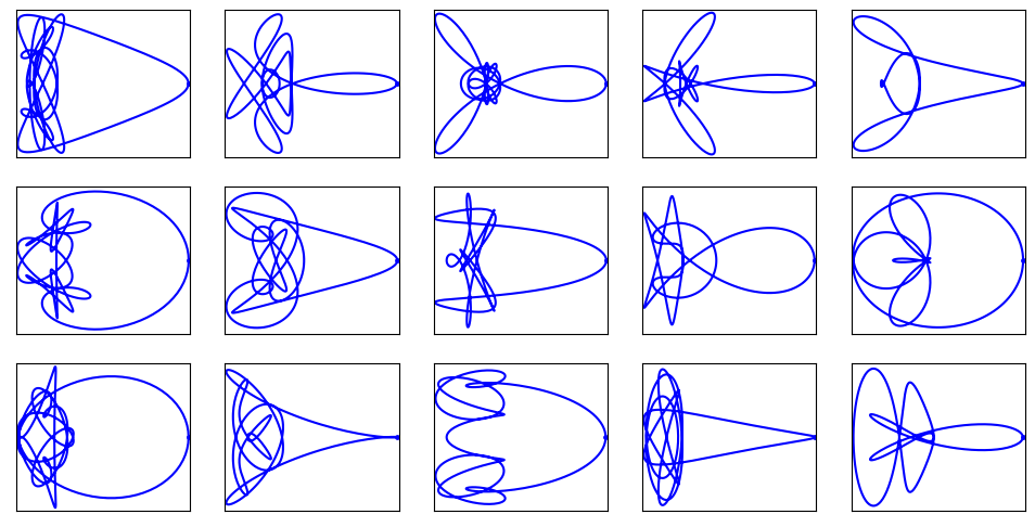
We pick random \(\mathbf{C} \in \mathbb{R}^{2N+1}\) (see, its real numbers now) and run the clock \(t=0\rightarrow 1\) and trace the path travelled by the complex point \(f(t, \mathbf{C}) \in \mathbb{C}\) as time progresses. It creates patterns like the ones shown below
There is one way to customize these - the value of \(N\). As we know that \(c_n\) has the interpretation of the magnitude of \(n^{th}\) frequency component. A large value of \(N\) implies the introduction of more high frequency into the time-domain signal. This visually leads to \(f(t)\) having finer details (i.e., more curves and bendings). Lowering the value of \(N\) would clear out these fine details and the path will become more and more flat. The below image shows decreasing value of \(N = 10 \rightarrow 6\) along columns. You can see the patterns losing details as we go right. And just like before, every run will create different patterns as they are solely controlled by random numbered coefficients.
Want to learn more ?
Mandelbrot & Julia set
These two sets are very important in the study of “Fractals” - objects with self-repeating patterns. Fractals are extremely popular concepts in certain branches of mathematics but they are mostly famous for having eye-catching visual appearance. If you ever come across an article about fractals, you are likely to see some of the most artistic patterns you’ve ever seen in the context of mathematics. Diving into the details of fractals and self-repeating patterns will open a vast world of “Mathematical Art”. Although, in this article, I can only show you a tiny bit of it - two sets namely “Mandelbrot” and “Julia” set. Let’s start with the all important function
\[ f_C(z) = z^2 + C \]
where \(C, f_C(z), z \in \mathbb{C}\) are complex numbers. This appearantly simply complex-valued function is in the heart of these sets. All it does is squares its argument and adds a complex number that the function is parameterized with. Also, we denote \(f^{(k)}_C(z)\) as \(k\) times repeated application of the function on a given \(z\), i.e.
\[ f^{(k)}_C(z) = f_C(\cdots f_C(f_C(z))) \]
Mandelbrot Set
With these basic definitions in hand, the Mandelbrot set (invented by mathematician Benoit Mandelbrot) is the set of all \(C\in\mathbb{C}\) for which \[ \lim_{k\rightarrow\infty} \vert f^{(k)}_C(0+0j) \vert < \infty \]
Simply put, there is a set of values for \(C\) where if you repeatedly apply \(f_C\) on zero (i.e. \(0+0j\)), the output does not diverge. All such values of \(C\) makes the so called “Mandelbrot Set”. For the values of \(C\) that does not diverge, can be characterized by how many repeated application of \(f_C(\cdot)\) they can tolerate before their absolute value goes higher than a predefined “escape radius”, let’s call it \(r\in\mathbb{R}\). This creates a loose sense of “strength” of a certain \(C\) that can be written as
\[ \mathbb{K}(C) = \max_{\vert f^{(k)}_C(0+0j) \vert \leq r} k \]
It might look all strange but if you treat the integer \(\mathbb{K}(C)\) as grayscale intensity value for a grid of points on 2D complex plane (i.e., an image), you will get a picture similar to this (Don’t get confused, the picture is indeed grayscale; I added PyPlot’s plt.cm.twilight_shifted colormap for enhancing the visual appeal). The grid is in the range \((-2.5+1.5j) \rightarrow (1.5-1.5j)\) and the escape radius is \(r=2.5\).
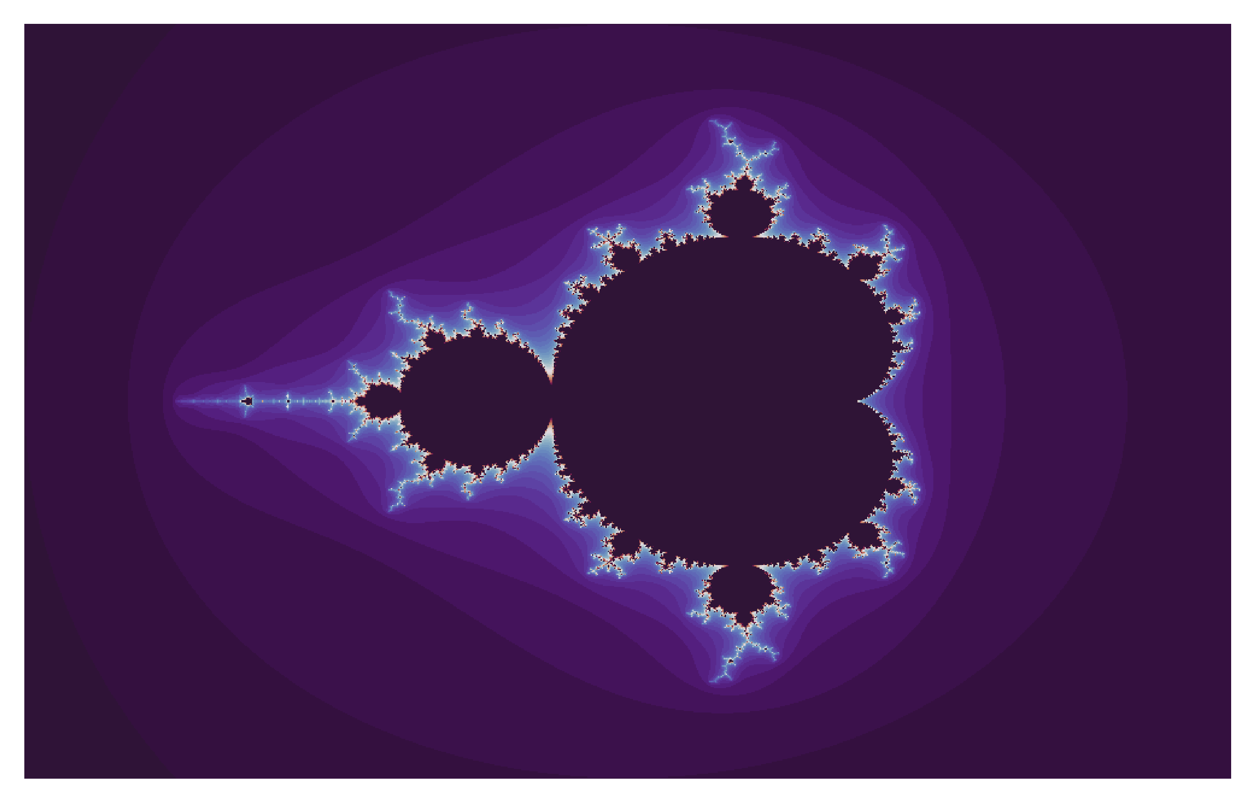
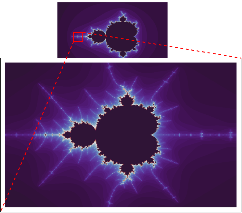
What is so fascinating about this pattern is the fact that it is self-repeating. If you zoom into a small portion of the image, you would see the same pattern again.
Julia Set
Another very similar concept exists, called the “Julia Set” which exhibits similar visual \(\mathbb{K}\) diagram. Unlike Mandelbrot set, we consider a \(z\in\mathbb{C}\) to be in Julia set \(\mathbf{J}_C\) if
\[ \lim_{k\rightarrow\infty} \vert f^{(k)}_C(z) \vert < \infty \]
Please note that this time the set is parameterized by \(C\) and we are interested in how the argument of the function behaves under repeated application of \(f_C(\cdot)\). Now things from here are similar. We define a similar “strength” for every \(z\in\mathbb{C}\) as
\[ \mathbb{K}\_C(z) = \max_{\vert f^{(k)}\_C(z) \vert \leq r} k \]
Please note that as a result of this new definition, the \(\mathbb{K}\) diagram is parameterized by \(C\), i.e., we will get different image for different \(C\). In principle, we can visualize such images for different \(C\) (they are indeed pretty cool), but let’s go a bit further than that. We will vary \(C\) along a trajectory and produce the \(\mathbb{K}\) diagrams for each \(C\) and see them as an animation. This creates an amazing visual effect. Technically, I varied \(C\) along a circle of radius \(R = 0.75068\), i.e., \(C = R e^{j\theta}\) with \(\theta = 0\rightarrow 2\pi\)
Want to know more ?
Alright then ! That is pretty much it. Due to constraint of time, space and scope its not possible to explain everything in detail in one article. There are plenty of resources available online (I have already provided some link) which might be useful in case you are interested. Feel free to explore the details of whatever new you learnt today. If you would like to reproduce the diagrams and images, please use the code here https://github.com/dasayan05/patterns-of-randomness (sorry, the code is a bit messy, you have to figure out).
Citation
@online{das2020,
  author = {Das, Ayan},
  title = {Patterns of {Randomness}},
  date = {2020-04-15},
  url = {https://ayandas.me/blogs/2020-04-15-patterns-of-randomness.html},
  langid = {en}
}