Recently, Geoffrey Hinton, the godfather of deep learning argued that one of the key principles in the ConvNet model is flawed, i.e., they don’t work the way human brain does. Hinton also proposed an alternative idea (namely capsules), which he thinks is a better model of the human brain. In this post, I will try to present an intuitive explanation of this new proposal by Hinton and colleagues.
In the ongoing renaissance of deep learning, if we have to chose one specific neural network model which has the most contribution, it has to be the Convolutional Neural Networks or ConvNets as we call. Popularized by Yann LeCun in the 90’s, these models have gone through various modifications or improvements since then - be it from theoretical or engineering point-of-view. But the core idea remained more or less same.
The recent fuss about capsules really started just after the publication of the paper named Dynamic Routing Between Capsules by Sara Sabour, Nicholas Frosst and Geoffrey Hinton. But, it turned out that hinton had this idea way back in 2011 (Transforming Auto-encoders) but for some reason it didn’t catch much attention. This time it did. Equipped with the idea of capsules, hinton and team also achieved state-of-the-art performance on MNIST digit classification dataset.
This article is roughly divided into 3 parts:
- Description of the normal ConvNet model
- What hinton thinks is wrong in it
- The new idea of capsules
The usual ConvNet model
I will briefly discuss ConvNets here. If you are not well aware of the nitty-gritties of ConvNet, I would suggest reading a more detailed article (like this).
Convolutional neural networks are specially designed to exploit the 2D structure of images. Usual ConvNet architectures (Figure-1) have two core operations
2D convolution:
Convolution operation or filtering is running a 2D kernel (usually of size quite smaller than the image itself) spatially all over an image which looks for a specific pattern in the image and generates an activation map (or feature map) which shows the locations where it was able to spot the pattern (Figure-2). 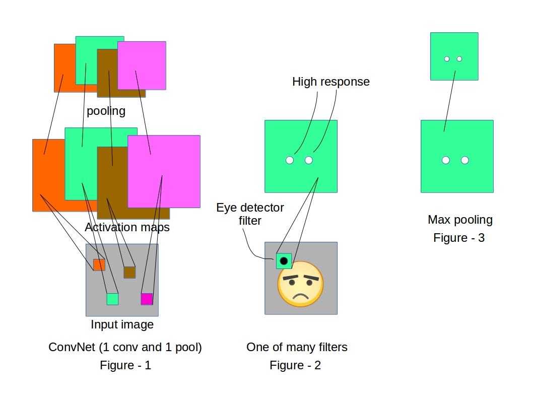
Pooling:
Most frequently used type of pooling, i.e. Max-pooling is used to reduce the size of the feature maps/activation maps (Figure-3) for computational benefit. But, it has one other purpose (which is exactly what Geoff Hinton has a problem with). The max-pooling is supposed to induce a small translation invariance in the learning process. If an entity in the image is translated by a small amount, the activation map corresponding to that entity will shift equally. But, the max-pooled output of the activation map remains unaltered. 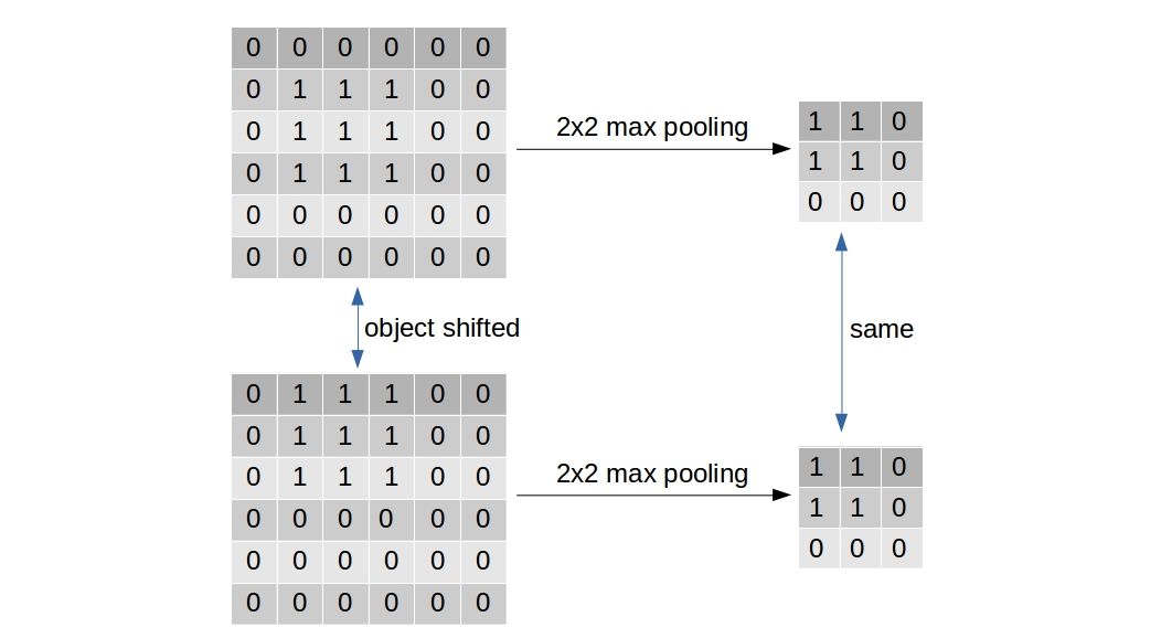
After stacking multiple convolution and pooling layers, usually all the neurons are flattened into one dimensional array and fed into a multilayer perceptron of proper depth and width.
Different layers of abstraction
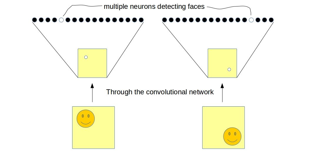
Trained with a supervised learning procedure, the network will be able to produce different levels of abstracted representation of a given image. For example, trained on a dataset with lots of facial images, a convnet will possibly learn to detect lower level features like edges, corners in its earliest layers. The layers above that will learn to detect smaller facial parts like eyes, noses etc. And the top most layer will be detecting whole faces. 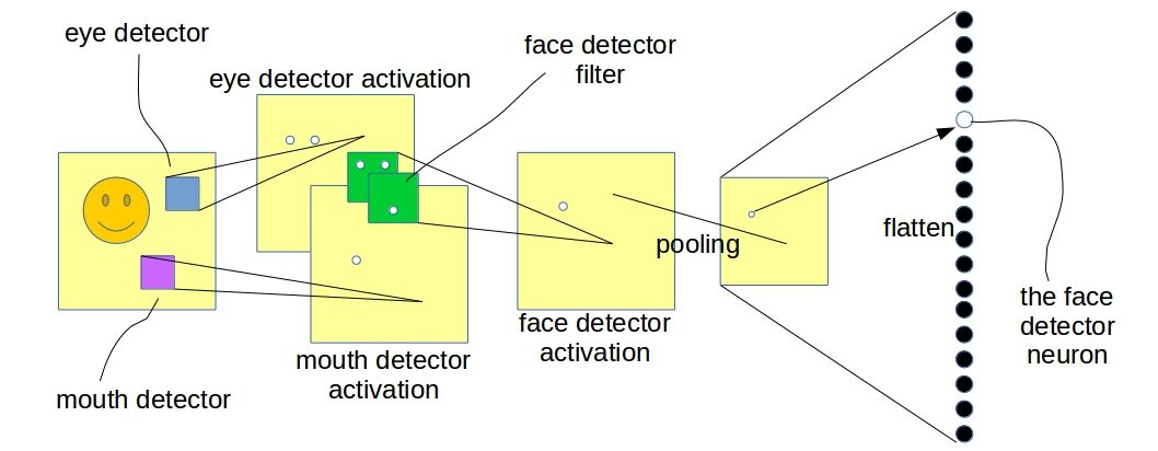
In the above illustration, the lower level convolutional layer is detecting facial parts and the layer above (the next convolutional layer) is detecting faces with the help of information from the layer below. The “white dots” in the image denote high responses in the activation map indicating a possible presence of the entity it was searching for. One thing to note, the above illustration is only a pictorial representation and does not exactly depict what a ConvNet learns in reality. The two convolutional layers in the figure can be any two successive layers in a deeper convnet.
What is wrong with ConvNets ?
Geoffrey Hinton, in his recent talks on capsules, argued that the present from of ConvNet is not a good representation of what happens in the human brain. Particularly, his disagreement is over the way ConvNet solves the invariance problem. As I earlier explained, pooling is primarily responsible for inducing translation invariance. The argument against pooling as stated by Hinton himself, is > max-pooling solves the wrong problem - we want equivariance, not invariance
How ConvNets do it - the “Place-coding”
Consider the network I showed in the last figure. Now we have training samples same as the one shown in the figure and also its translated version - translated by a significant amount so that it is well beyond the capability of the max-pooling layer to have the same activation map. In this case, the network will have two different neurons detecting the same face in two different locations.
If we consider the output of the flatten layer to be a codified representation of the image which we often do, it will be clear that the network is invariant to translation, i.e., the “two neurons” togather is able to predict whether a face is present in either location of the image. The problem with this approach is not only the fact that it is now the responsibility of multiple neurons to detect a single entity but also it is losing “explicit pose information” (phrase coined by hinton). Although one must realize that there are implicit informations in the network in the form of “relative activations of neurons” about the location of the entity (face in this case) in image. This is what neuroscientists call the place-coding.
How human brain does it - the “Rate-coding”
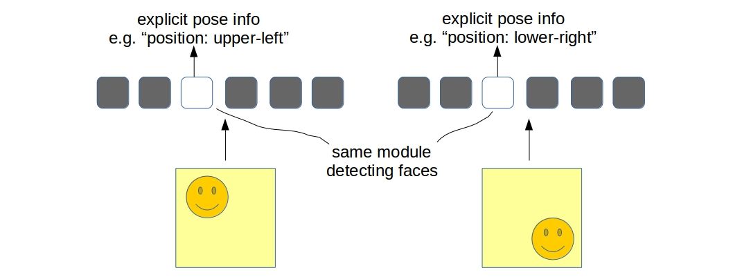
The brain also represents an image with several layers of abstraction but according to Hinton’s hypothesis, it learns to detect entities in each layer with equivariance. What it means is, the brain contains some “modules/units” for detecting different entities - just one for each entity. Such modules/units have the ability to “explicitly represent” the “pose” of an entity. This is called the rate-coding. Clearly, a scalar neuron is not enough to avail such representational power.
The resemblance with computer graphics
Geoff Hinton often draws a comparison between “human vision system” with “computer graphics” by saying > human brain does the opposite of computer graphics
I will try to explain what he means by that. In a typical computer graphics rendering system we present a 3D model with a set of vertices/edges (which we often call a mesh) and it gets converted into a 2D image which can then be visualized on computer screens. How humans do visual perception is pretty much the opposite - it figures out the “explicit pose informations” about an entity from the 2D image and reverts it to get the mesh back. This notion of extracting “explicit pose information” resembles quite well with the new “modules/units” that I have talked about in the previous section.
The new idea of Capsules
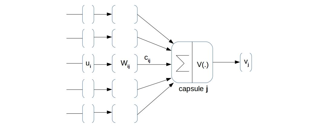
As I stated earlier, a neuron-model that spits out a scalar value is certainly not enough to represent explicit pose of an entity. This is where Hinton and team came up with the idea of capsules which is nothing but an extension to the familiar neuron-model. > A capsule is basically a “vector-neuron” which takes in a bunch of vectors and produces a single vector. They are simply “vector-in-vector-out” computation units.
These are the mathematical notations I’m gonna use here onwards:
- \(\displaystyle{ u_i \in \mathbb{R}^n}\): the \(i^{th}\) input vector of dimension \(n\) for \(i=1,2,...,I\)
- \(\displaystyle{ v_j \in \mathbb{R}^d}\): the output vector of dimension \(d\) for \(j=1,2,...,J\)
- \(\displaystyle{ W_{ij} \in \mathbb{R}^{n \times d}}\): the weight matrix between capsule \(i\) of layer \(l\) and capsule \(j\) of layer \(l+1\) *\(\displaystyle{ c_{ij} \in \mathbb{R}}\): the coupling coefficients between capsule \(i\) of layer \(l\) and capsule \(j\) of layer \(l+1\). I’ll come to this later in detail.
The pre-activation of capsule \(j\) is given by $ $ where \(\displaystyle{ \hat{u_{ij}} = W_{ij} u_i }\). Then the activation is given by \(\displaystyle{ v_j = V( s_j ) }\) where \(V()\) is a “vector nonlinearity”. The \(\displaystyle{ \hat{u_{ij}} }\) is called “prediction vector” from capsule \(i\) of layer \(l\) to capsule \(j\) of layer \(l+1\).
The authors of the paper presented one particular vector non-linearity $ $ which worked in their case but it certainly is not the only one. Considering the fast pace in which the deep learning community works, it won’t take too long to come up with new and improved vector non-linearities.
How does this help ?
Equipped with the mathematical model of capsules, we now have a way to represent “explicit pose parameters” of an entity. One capsule in any layer is a dedicated unit for detecting a single entity. If the pose of the entity changes (shifts, rotates, etc.), the same capsule will remain responsible for detecting that entity just with a change in its activity vector (\(v_j\)). For example, a capsule detecting a face might output an activity vector \(v_j = [0.5, 0.2]\) which when rotated outputs \(v_j = [0.3, 0.46]\). Additionally, the length of the vector (euclidean distance of the vector from origin) represents the probability of existence of that entity. The kind of vector non-linearity used in the capsule model will ensure that the length of vector lie between 0 and 1 (interpreted as probability).
Although we now have a structurally different neuron model, two consecutive capsule layers will still learn two levels of abstracted representation just like normal ConvNet.
But as we now have more representation power in a single neuron (namely capsule), we should exploit it to ensure a meaningful information flow between two neurons of successive layers. Such parametric structure (\(W_{ij}\) and \(c_{ij}\)) of capsule has been carefully designed to do exactly that. The reader is advised to take extra care in understanding the next two sub-sections because they are the heart of the idea of capsules.
Interpretation of \(W_{ij}\) :
\(\displaystyle{W_{ij} \in \mathbb{R}^{n \times d}}\) is a model parameter and learned by a supervised training process just like the connections in the normal neural networks. But, they have a quite different interpretation than that of the scalar neurons. Activities (\(u_i\)) of each capsule in the lower level gets matrix-multiplied by \(W_{ij}\) and produces what the authors of the paper call “prediction vectors” (\(\displaystyle{ \hat{u_{ij}} }\)). There is a reason for such a name.
\(W_{ij}\) basically performs an “affine transform” on the incoming capsule activations (\(u_i\) - pose parameters of lower level entities) and makes a “guess” about what the activities of the higher level capsules (\(v_j\)) could be.
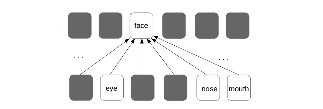
In our running example of face detection, the activity vector (pose parameters) of the eye detector capsule (let’s call it \(\displaystyle{ u_e }\)) makes a prediction \(\displaystyle{ \hat{u_{ef}} = W_{ef} u_{e} }\) which is nothing but a guess of \(\displaystyle{ v_{f} }\), the activity of the face detector capsule (i.e., the pose of the face) in the next layer.
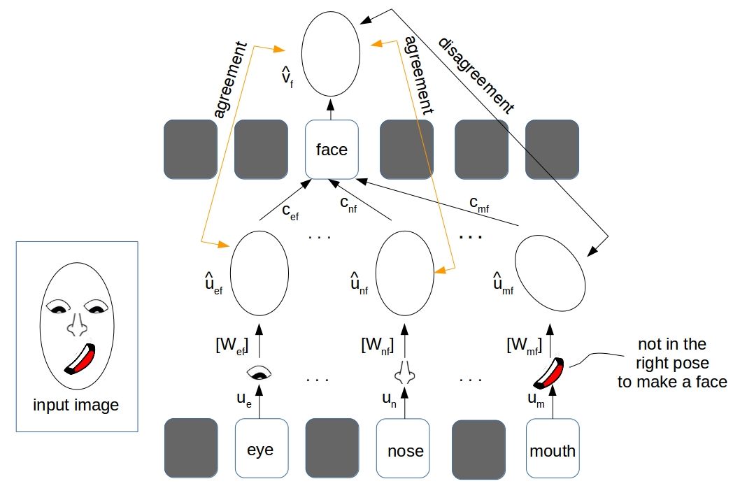
As shown in the illustration above, the pose vectors of the eye, nose and mouth (\(u_e\), \(u_n\) and \(u_m\)) detector capsules in the lower level layer individually predicted possible poses of the face( \(\displaystyle{\hat{u_{ef}}}\), \(\displaystyle{\hat{u_{nf}}}\) and \(\displaystyle{\hat{u_{mf}}}\)). The mouth detector in the figure needs some extra attention as it has predicted the face pose which does not “aligns” with the real face pose in the input image. To sum it up, the parameters \(W_{ij}\) models a “part-whole” relationship between the lower and higher level entities (or capsules).
Interpretation of \(c_{ij}\) and the “Dynamic Routing”:
If you understood the previous sub-section properly, it should be clear by now that there can be some lower level prediction vectors which won’t “align” with the higher level capsule activities indicating that they are not related by a “part-whole” relationship. In the paper “Dynamic Routing Between Capsules” the authors have proposed a way to “de-couple” the connection between such capsules.
The process is fairly simple: take a prediction vector \(\displaystyle{\hat{u_{ij}}}\) from the lower level and an activity vector \(v_j\) from next level and measure how much they agree by computing an “agreement” quantity \(\displaystyle{ a_{ij} = \langle \hat{u_{ij}}, v_j \rangle }\). Judging by the values of $ $, we can then “strengthen” or “weaken” the correspodning connection strength by highering or lowering \(\displaystyle{ c_{ij}}\) appropriately.
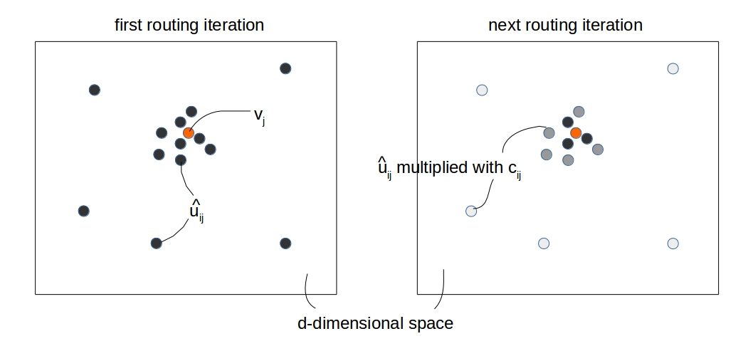
The process can be thought of collecting “high-dimensional votes” from all the capsules below and matching it with the top level capsule \(v_j\) and de-coupling the ones which don’t agree with it. By “fading away” the incoming connections that don’t agree, we enforce the connection parameters (\(W_{ij}\)) to learn more prominent “part-whole” relationships. In the figure below, the incoming “prediction vectors (\(\hat{u_{ij}}\))” for a specific \(j\) is shown for two consecutive iterations. The intensity of the grey color denotes the “degree of contribution” of a particular \(\hat{u_{ij}}\) towards the \(v_j\).
Having the “prediction vectors (\(\displaystyle{\hat{u_{ij}}}\))” available, the exact way of doing dynamic routing is as follows:
- set \(b_{ij} \leftarrow 0\) for a single training sample
- for \(r = 1 \rightarrow R\):
- compute \(c_{ij} = softmax(b_{ij})\) over all \(j\)
- compute \(s_j\) and \(v_j\) according to the capsule-model equations
- compute “agreement” \(a_{ij}\) between \(v_j\) and \(\hat{u_{ij}}\)
- update \(b_{ij}^{new} \leftarrow b_{ij}^{old} + a_{ij}\)
- take \(v_j\) at the end of \(R\) routing iterations
Now couple of things to note here:
- \(c_{ij}\) is the true coupling coefficient. Having an intermediate \(b_{ij}\) makes sure \(\sum_j c_{ij} = 1\)
- We compute the \(c_{ij}\) for each training sample. \(c_{ij}\) is not a global model parameter, it resets to initial for each sample whlie training
- We execute the routing in the process of computing \(v_j\). \(v_j\) is the end product of \(R\) iterations of routing
- We usually take \(R\) to be \(2 \rightarrow 5\)
So, that brings us to the end of the general discussion on capsules. In the next article, I will explain the specific CapsNet architecture (with tensorflow implementation) that has been used for MNIST digit classification task. See you.
Citation
@online{das2017,
  author = {Das, Ayan},
  title = {An Intuitive Understanding of {Capsules}},
  date = {2017-11-20},
  url = {https://ayandas.me/blogs/2017-11-20-an-intuitive-understanding-of-capsules.html},
  langid = {en}
}