While a plethora of high-quality text-to-image diffusion models (Ramesh et al. 2022; Rombach et al. 2022; Podell et al. 2024) emerged in the last few years, credit mostly goes to the tremendous engineering efforts put into them. The fundamental theory behind them however, remained largly untouched – well, untill recently. The traditional “markov-chain” (Ho et al. 2020) or “SDE” (Song et al. 2021) perspective is now being replaced by an arguably simpler and flexible alternative. Under the new approach, we ditch the usual notion of a stochastic mapping as the model and adopt a deterministic mapping instead. Turns out that such model, although existed, never took off due the absense of a scalable learning algorithm. In this article, we provide a relatively easy and visually guided tour of “Flow Matching”, followed by ideas like “path straightening” & “reflow”. It is worth mentioning that this very idea powered the most recent version of Stable Diffusion (i.e. SD3 by Esser et al. (2024)).
Every scalable generative model follows a “sampling first” philosophy, i.e. they are defined in terms of a (learnable) mapping (say \(F_{\theta}\)), which maps (known) pure noise \(z\) to desired data \(x\)
\[ x = F_{\theta}(\epsilon), \text{ where } \epsilon \sim \mathcal{N}(0, I) \tag{1}\]
The learning objective is crafted in a way that the \(F_{\theta}\) induces a model distribution on \(x\), i.e. \(p_{\theta}(x)\) that matches a given \(q_{data}(x)\) as closely as possible. That is, of course, from the samples of \(q_{data}(x)\) only. Different generative model families learn (parameters of) the mapping in different ways.
Brief overview of Diffusion Models
The generative process
Although there are mutiple formalisms to describe the underlying theory of Diffusion Models, the one that gained traction recently is the “Differential Equations” view, mostly due to Song et al. (2021). Under this formalism, Diffusion’s generative mapping (in Equation 1) can be realized by integrating a differential equation in time \(t\). Song et al. (2021) also showed that there are two equivalent generative processes, one stochastic and another deterministic, that leads to exact same noise-to-data mapping.
\[ dx_t = \Big[f(t) x_t - g^2(t) \underbrace{\nabla_{x_t} \log p_t(x_t)}_{\approx s_{\theta}(x_t, t)} \Big] dt + g(t) d\bar{w} \tag{2}\] The hyper-parameters \(f(t)\) and \(g(t)\) are scalar functions of time.
\[ dx_t = \Big[f(t) x_t - {\color{blue}0.5}\ \cdot g^2(t) \underbrace{\nabla_{x_t} \log p_t(x_t)}_{\approx s_{\theta}(x_t, t)} \Big] dt \cancel{+ g(t) d\bar{w}} \tag{3}\] The hyper-parameters \(f(t)\) and \(g(t)\) are scalar functions of time.
where \(p_t(x_t)\) is a noisy version of the data density1 induced by a (known & fixed) forward process over time \(t\)
1 Knowns as the forward process marginal
\[ dx_t = f(t)x_t dt + g(t) dw \]
\[ x_t = \alpha(t) x_0 + \sigma(t) \epsilon \tag{4}\]
\[ p_t(x_t | x_0) = \mathcal{N}(x_t; \alpha(t) x_0, \sigma(t)^2 \mathrm{I}) \]
The relationship between \(\{ f(t), g(t) \}\) and \(\{ \alpha(t), \sigma(t) \}\) is as follows.
\[ f(t) = \frac{d}{dt} \log \alpha(t), \text{ and } g(t)^2 = - 2 \sigma(t)^2 \frac{d}{dt} \log \frac{\alpha(t)}{\sigma(t)} \tag{5}\]
Despite being able sample \(x_t\) using Equation 4, the quantity \(\nabla_{x_t} \log p_t(x)\)2 in Equation 2 or Equation 3 is not analytically computable and therefore learned using a neural function.
2 The ‘score’ of the marginal
The learning objective
A parametric neural function \(s_{\theta}(x_t, t)\) is regressed using a different regression target than the ‘true’ target
\[ \mathcal{L}(\theta) = \mathbb{E}_{t, x_0 \sim q_{data}(x), x_t \sim p_t(x_t | x_0)} \Big[ || s_{\theta}(x_t, t) - \nabla_{x_t} \log p_t(x_t | x_0) ||^2 \Big] \tag{6}\] This objective is known as “Denoising Score Matching” (Vincent 2011).
\[ \mathcal{L}(\theta) = \mathbb{E}_{t, x_0 \sim q_{data}(x), x_t \sim p_t(x_t | x_0)} \Big[ || s_{\theta}(x_t, t) - \nabla_{x_t} \log p_t(x_t) ||^2 \Big] \tag{7}\] This is the true objective that is not directly computable.
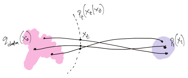
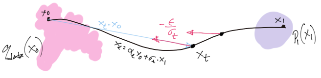
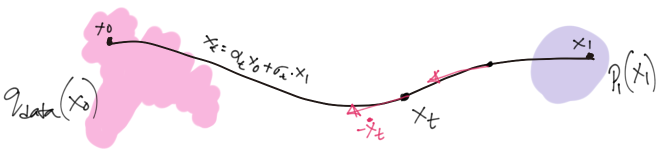
It was proved initially by Vincent (2011) and later re-established by Song et al. (2021) that using \(\nabla_{x_t} \log p_t(x_t | x_0)\)3 (in Equation 6) as an alternative target for regression can still lead to an ubiased estimate of the true \(\nabla_{x_t} \log p_t(x_t)\). The figure below show graphically, the quantity (red arrows) our parametric score model regresses against at an arbitrary timestep \(t\).
3 Please note that \(\nabla_{x_t} \log p_t(x_t | x_0) = - \frac{x_t - x_0}{\sigma^2_t} = - \frac{\epsilon}{\sigma_t}\)
Matching flows, not scores
The idea of re-interpreting reverse diffusion as “flow”4 stems from a holistic observation. Note that given Equation 3, an ODE dynamics is guaranteed to exists which induces a deterministic mapping from noise to any given data distribution. In diffusion model’s framework, we were only learning a part of the dynamics – not the dynamics itself.
4 This term comes from Continuous Normalizing Flows (CNFs)
\[ dx_t = \Bigg[ \underbrace{f(t) x_t - 0.5\ \cdot g^2(t) \overbrace{s_{\theta}(x_t, t)}^{\text{Instead of this ..}}}_{\text{.. why not learn this ?}} \Bigg] dt \tag{8}\]
A deterministic model
Following the observation above, we can assume a generative model realized by a deterministic ODE simulation, whose parametric dynamics subsumes \(f(t), g(t)\) and the parametric scores \(s_{\theta}(x_t, t)\)
\[ dx_t = v_{\theta}(x_t, t) dt, \text{ where } x_1 := \epsilon \sim \mathcal{N}(0, I) \tag{9}\]
Turns out, models like Equation 9 have already been investigated in generative modelling literature under the name of Continuous Normalizing Flows (Chen et al. 2018). However, these models never made it to the scalable realm due to their “simulation based”5 learning objective. The dynamics is often called “velocity”6 or “velocity field” and denoted with \(v\).
5 One must integrate or simulate the ODE during training.
6 It is a time derivative of position.
7 .. or as it is now called, the ‘Flow Matching’ loss
Upon inspecting the pair of Equation 8 and Equation 6, it is not particularly hard to sense the existance of an equivalent ‘velocity matching’ loss7 for the new flow model in Equation 9.
An equivalent objective
To see that exact form of the flow matching loss, simply try recreating the ODE dynamics in Equation 8 within Equation 6 by appending some extra terms that cancel out
\[ \begin{split} \mathcal{L}(\theta) = \mathbb{E}_{t, x_0 \sim q_{data}(x), x_t \sim p_t(x_t | x_0)} &\Bigg[ \left|\left| \frac{2}{g^2(t)} \left\{ \left( f(t) x_t - \frac{1}{2} g^2(t) s_{\theta}(x_t, t) \right) \right. \right. \right. \Bigg. \\ &\ \ \ \ \ \ \ \ \ \ \ \ \ \Bigg. \left. \left. \left. - \left( f(t) x_t - \frac{1}{2} g^2(t) \nabla_{x_t} \log p_t(x_t | x_0) \right) \right\} \right|\right|^2 \Bigg] \end{split} \]
The expression within the first set of parantheses ( .. ) is equivalent to what now call the parametric velocity/flow or \(v_{\theta}(x_t, t)\). The expression in second set of parantheses is a proxy regression target (let’s call it \(v(x_t, t)\)), equivalent to \(\nabla_{x_t} \log p_t(x_t | x_0)\) in score matching (see Equation 6). With the help of \(\{ f, g \} \rightleftarrows \{ \alpha, \sigma \}\) conversion (see Equation 5), it’s relatively easy to show that \(v(x_t, t)\) can be written as the time-derivative of the forward sampling process
\[ \begin{aligned} v(x_t, t) &\triangleq f(t) x_t - \frac{1}{2} g^2(t) \nabla_{x_t} \log p_t(x_t | x_0) \\ &= f(t)(\alpha(t) x_0 + \sigma(t) \epsilon) - \left[- \sigma(t) \frac{g(t)^2}{2 \sigma(t) } \frac{\epsilon}{\sigma(t)} \right] \\ &= \frac{\dot{\alpha}(t)}{\alpha(t)}(\alpha(t) x_0 + \sigma(t) \epsilon) - \left[ \sigma(t) \left( \frac{\dot{\alpha}(t)}{\alpha(t)} - \frac{\dot{\sigma}(t)}{\sigma(t)} \right) \epsilon \right] \\ &= \dot{\alpha}(t) x_0 + \cancel{\frac{\dot{\alpha}(t)}{\alpha(t)} \sigma(t) \epsilon} - \cancel{\sigma(t) \frac{\dot{\alpha}(t)}{\alpha(t)} \epsilon} + \dot{\sigma}(t) \epsilon \end{aligned} \]
\[ v(x_t, t) = \dot{\alpha}(t) x_0 + \dot{\sigma}(t) \epsilon = \dot{x}_t \]
To summarize, the following is the general form of flow matching loss
\[ \mathcal{L}_{FM}(\theta) = \mathbb{E}_{t, x_0 \sim q_{data}(x), x_t \sim p_t(x_t | x_0)} \Bigg[ \Bigg|\Bigg| v_{\theta}(x_t, t) - (\underbrace{\dot{\alpha}(t) x_0 + \dot{\sigma}(t) \epsilon}_{\dot{x}_t}) \Bigg|\Bigg|^2 \Bigg] \tag{10}\]
In practice, as proposed by many (Lipman et al. 2022; Liu et al. 2022), we discard the weightning term just like Diffusion Model’s simple loss popularized by Ho et al. (2020). We may think of \(\dot{x}_t\) as a stochastic velocity induced by the forward process. The model, when minimized with Equation 10, tries to mimic the stochastic velocity, but without having access to \(x_0\).
While the learning objective regresses against \(\dot{x}_t\), we need \(-\dot{x}_t\) for sampling. The extra negative is induced automatically while simulating Equation 9 in reverse time (\(dt\) being negative). It is therefore equivalent to think the regression target to be \(-\dot{x}_t\).
The minima & its interpretation
The loss in Equation 10 can be shown to be equivalent8 to
8 Their gradients are equal, but the losses are not.
\[ \mathcal{L}_{FM}(\theta) = \mathbb{E}_{t, x_t \sim p_t(x_t)} \Bigg[ \Bigg|\Bigg| v_{\theta}(x_t, t) - \mathbb{E}_{x_0 \sim p(x_0|x_t)} \big[\dot{x}_t\big] \Bigg|\Bigg|^2 \Bigg] \tag{11}\]
which implies that the loss reaches its minima9 when the model perfectly learns
9 This is a typical MMSE estimator.
\[ v_*(x_t, t) \triangleq \mathbb{E}_{x_0 \sim p(x_0|x_t)} \left[\dot{x}_t\right] \]
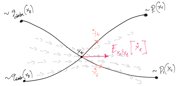
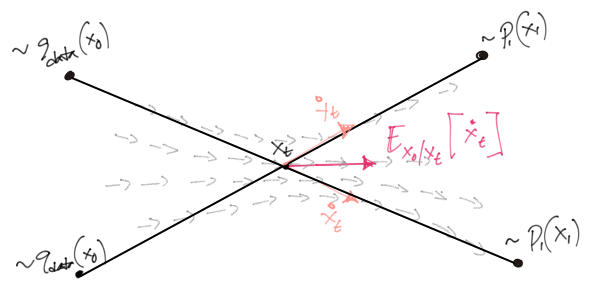
Hence, \(v_{\theta}\) can be regarded as the variational approximation of the posterior velocity \(v_*\). Note that \(v_*\) is non-causal, i.e. it has access to the true data distribution \(q_{data}(x_0)\). On the other hand, the model \(v_{\theta}\) must be causal. Hence, the learning process “causalizes” (Liu et al. 2022) the stochastic path.
The forward stochastic paths \(x_t\) are also overlapping, while the model is a function10. The expectation \(\mathbb{E}_{x_0 \sim p(x_0|x_t)} \left[ \cdot \right]\) averages the stochastic velocity over all possible real data points \(x_0 | x_t\), leading to smooth velocity fields learned by the model.
10 cannot have multiple value at one given point
The optimally learned generative process (Equation 9) can therefore be expressed as
\[ dx_t = v_{*}(x_t, t) dt, \text{ where } x_1 := \epsilon \sim \mathcal{N}(0, I) \]
Straightening & ReFlow
\(t\)-independent stochastic velocity
With the general theory understood, it is now easy to concieve the idea of straight flows. It simply refers to the following special case
\[ \alpha(t) = 1 - t, \sigma(t) = t \]
which implies the forward process and its time derivative to be
\[ \begin{aligned} x_t &= (1 - t) \cdot x_0 + t \cdot x_1 \\ \implies \dot{x}_t &= - x_0 + x_1 \end{aligned} \]
What is important is the stochastic velocity is independent of time11 and the \(x_t\) trajectory itself is a stright line.
11 Not “constant” – it still depends on data \(x_0\) and noise sample \(\epsilon\), which are random variables.
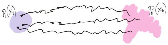
This however, does not mean that the learned model will produce straight paths – it only means we’re supervising the model to follow a path as straight as possible. An analogous illustration was provided in Liu et al. (2022) which is a bit more descriptive.

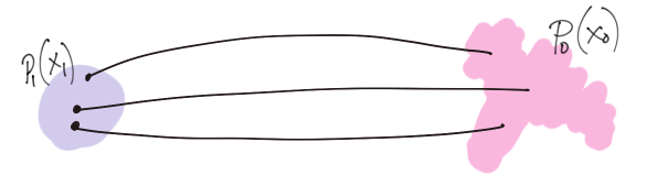
This learning problem (Equation 11) effectively turns an independent stochastic ‘coupling’ \(q_{data}(x_0) \mathcal{N}(x_1; 0, I)\) into a deterministic coupling \(p(z_0, z_1)\) with some dependence. This prcoess \((x_0, x_1) \rightarrow (z_0, z_1)\) has been termed (by Liu et al. (2022)) as “Rectification”. Samples from this deterministic coupling can be drawn by drawing noise sample \(z_1 := \epsilon \sim \mathcal{N}(\epsilon; 0, I)\) and then simulating the flow in Equation 9 with the learned model
\[ z_0 = z_1 + \int_{t=1}^{t=0} v_{\theta}(z_t, t) dt. \]
It can be proved that the samples \((z_0, z_1)\) are, in average, closer to each other than that of \((x_0, x_1)\).
\[ \begin{aligned} \mathbb{E}_{p(z_0, z_1)} \left[ || z_0 - z_1 || \right] &= \mathbb{E}_{p(z_0, z_1)} \left[ || \int_{1}^{0} v_{*}(z_t, t) dt || \right] \\ &\leq \mathbb{E}_{p(z_0, z_1)} \left[ \int_{1}^{0} || v_{*}(z_t, t) || dt \right] \\ &= \mathbb{E}_{p(x_0, x_1)} \left[ \int_{1}^{0} || v_{*}(x_t, t) || dt \right] \\ &= \mathbb{E}_{p(x_0, x_1)} \left[ \int_{1}^{0} || \mathbb{E}[\dot{x}_t | x_t] || dt \right] \\ &\leq \mathbb{E}_{p(x_0, x_1)} \left[ \int_{1}^{0} \mathbb{E}[\ || \dot{x}_t ||\ |\ x_t] dt \right] \\ &= \int_{1}^{0} \mathbb{E}_{p(x_0, x_1)} \left[ \mathbb{E}[\ || x_0 - x_1 ||\ |\ x_t] \right] dt \\ &= \mathbb{E}_{p(x_0, x_1)} \left[ || x_0 - x_1 || \right] \end{aligned} \]
The proof uses the following
- The fact that \(|| \cdot ||\) is a convex cost function.
- Convex functions can be exchanged with \(\mathbb{E}\) according to Jensen’s inequality.
- \(z_t\) and \(x_t\) has the same marginal and can be exchanges as a random variable.
- Assumes our model learns the perfect \(v_*\).
- Law of iterated expectation.
Please see section 3.2 of Liu et al. (2022) for more details on the proof.
Reflow
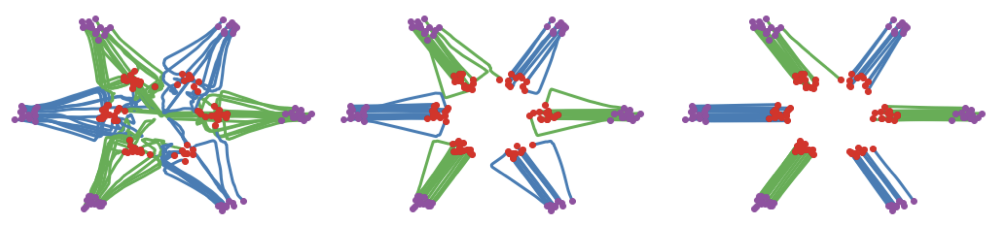
The process of rectification however, does not guarantee (as you can see in the above figure) the new coupling to have straight paths between each pair. Liu et al. (2022) suggested the “Reflow” procedure, which is nothing but learning a new model using the samples of \(p(z_0, z_1)\).
\[ \mathcal{L}_{FM}(\phi) = \mathbb{E}_{t,\ (z_0, \epsilon) \sim p(z_0, \epsilon)} \Big[ \Big|\Big| v_{\phi}(z_t, t) - (-z_0 + \epsilon) \Big|\Big|^2 \Big] \]
The ‘reflow’-ed coupling \((z_2, \epsilon)\) is guaranteed to have paths straighter than \((z_1, \epsilon)\). One can, in fact, repeat this procedure as many times as they want. Another figure from Liu et al. (2022) perfectly demonstrates successive reflows
In this article, we talked about Flow Matching, Rectification and Reflow – some of the emerging new ideas in Diffusion Model literature. Specifically, we looked into the theoretical definitions and justifications behind the ideas. Despite having an appealing outlook, some researchers are skeptical of it being a special case of good old Diffusion Models. Whatever the case maybe, it did deliver one of the best text-to-image model so far (Esser et al. 2024), pehaps with a bit of clever engineering, which is a topic of another day.
References
Citation
@online{das2024,
  author = {Das, Ayan},
  title = {Match Flows, Not Scores},
  date = {2024-04-26},
  url = {https://ayandas.me/blogs/2024-04-26-flow-matching-strightning-sd3.html},
  langid = {en}
}