Deep Learning at scale: The “torch.distributed” API

In the last post, we went through the basics of Distributed computing and MPI, and also demonstrated the steps of setting up a distributed environment. This post will focus on the practical usage of distributed computing strategies to accelerate the training of Deep learning (DL) models. To be specific, we will focus on one particular distributed training algorithm (namely Synchronous SGD) and implement it using PyTorch’s distributed computing API (i.e., torch.distributed). I will use 4 nodes for demonstration purpose, but it can easily be scaled up with minor changes. This tutorial assumes the reader to have working knowledge of Deep learning model implementation as I won’t go over typical concepts of deep learning.

Types of parallelization strategies :

There are two popular ways of parallelizing Deep learning models:

1. Data parallelism
2. Model parallelism

Let’s see what they are.

Model parallelism

Model parallelism refers to a model being split into two parts, i.e., some layers in one part and some in other, then execute it by placing them on different hardwares/devices. In this strategy, we typically start with one single piece of data and pass it through the parts one by one. Although placing the parts on different devices does have execution benefits (asynchronous processing of data), it is usually employed to avoid memory constraint. Models with very large number of parameters, which are difficult fit into a single system due to high memory footprint, benefits from this type of strategy.

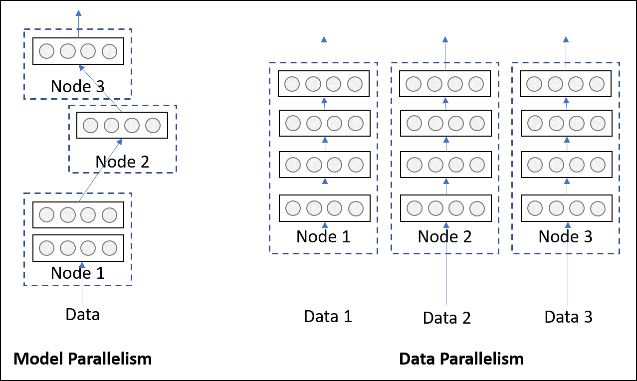
Data parallelism

Data parallelism, on the other hand, refers to processing multiple pieces (technically batches) of data through multiple replicas of the same network located on different hardwares/devices. Unlike model parallelism, each replica may be an entire network and not a part of it. This strategy, as you might have guessed, can scale up well with increasing amount of data. But, as the entire network has to reside on a single device, it cannot help models with high memory footprints. The illustration above (taken from here) should make it clear.

Practically, Data parallelism is more popular and frequently employed in large organizations for executing production quality DL training algorithms. So, in this tutorial, we will fix our focus on data parallelism.

The torch.distributed API :

Okay ! Now it’s time to learn the tools of the trade - PyTorch’s torch.distributed API. If you remember the lessons from the last post, which you should, we made use of the mpi4py package which is a convenient wrapper on top of original Intel MPI’s C library. Thankfully, PyTorch offers a very similar interface to use underlying Intel MPI library and runtime. Needless to say, being a part of PyTorch, the torch.distributed API has a very elegant and easy-to-use design. We will now see the basic usage of torch.distributed and how to execute it.

First things first, you should check the availability of distributed functionality by

import torch.distributed as dist
if dist.is_available():
    # do distributed stuff ...

Let’s look at this piece of code, which should make sense without explanation given that you remember the lessons from my last tutorial. But I am going to provide a brief explanation in case it doesn’t.

# filename 'ptdist.py'
import torch
import torch.distributed as dist

def main(rank, world):
    if rank == 0:
        x = torch.tensor([1., -1.]) # Tensor of interest
        dist.send(x, dst=1)
        print('Rank-0 has sent the following tensor to Rank-1')
        print(x)
    else:
        z = torch.tensor([0., 0.]) # A holder for recieving the tensor
        dist.recv(z, src=0)
        print('Rank-1 has recieved the following tensor from Rank-0')
        print(z)

if __name__ == '__main__':
    dist.init_process_group(backend='mpi')
    main(dist.get_rank(), dist.get_world_size())

Executing the above code results in:

cluster@miriad2a:~/nfs$ mpiexec -n 2 -ppn 1 -hosts miriad2a,miriad2b python ptdist.py
Rank-0 has sent the following tensor to Rank-1
tensor([ 1., -1.])
Rank-1 has recieved the following tensor from Rank-0
tensor([ 1., -1.])

1. The first line to be executed is dist.init_process_group(backend) which basically sets up the software environment for us. It takes an argument to specify which backend to use. As we are using MPI throughout, it’s backend='mpi' in our case. There are other backends as well (like TCP, Gloo, NCCL).

2. Two parameters need to be retrieved: the rank and world size which exactly what dist.get_rank() and dist.get_world_size() do respectively. Remember, the world size and rank totally depends on the context of mpiexec. In this case, world size will be 2; miriad2a and miriad2b will be assigned rank 0 and 1 respectively.

3. x is a tensor that Rank 0 intend to send to Rank 1. It does so by dist.send(x, dst=1). Quite intuitive, isn’t it ?

4. z is something that Rank 1 creates before receiving the tensor. Yes ! you need an already created tensor of same shape as a holder for catching the incoming tensor. The values of z will eventually be replaced by the values in x.

5. Just like dist.send(..), the receiving counterpart is dist.recv(z, src=0) which receives the tensor into z.

Communication collectives:

What we saw in the last section is an example of “peer-to-peer” communication where rank(s) send data to specific rank(s) in a given context. Although this is useful and gives you granular control over the communication, there exist other standard and frequently used pattern of communication called collectives. A full-fledged explanation of these collectives is beyond the scope of this tutorial, but I will describe one particular collective (known as all-reduce) which is of interest to us in the context of Synchronous SGD algorithm.

The common collectives are: 1. Scatter 2. Gather 3. Reduce 4. Broadcast 5. All-reduce 6. etc.

The all-reduce collective

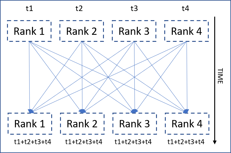
All-reduce is basically a way of synchronized communication where “a given reduction operation is operated on all the ranks and the reduced result is made available to all of them”. The above illustration hopefully makes it clear. Now, it’s time for some codes.

def main(rank, world):
    if rank == 0:
        x = torch.tensor([1.])
    elif rank == 1:
        x = torch.tensor([2.])
    elif rank == 2:
        x = torch.tensor([-3.])

    dist.all_reduce(x, op=dist.reduce_op.SUM)
    print('Rank {} has {}'.format(rank, x))

if __name__ == '__main__':
    dist.init_process_group(backend='mpi')
    main(dist.get_rank(), dist.get_world_size())

when launched in a world of 3, it produces

cluster@miriad2a:~/nfs$ mpiexec -n 3 -ppn 1 -hosts miriad2a,miriad2b,miriad2c python ptdist.py
Rank 1 has tensor([0.])
Rank 0 has tensor([0.])
Rank 2 has tensor([0.])

1. The same if rank == <some rank> .. elif pattern we encounter again and again. In this case, it is used to create different tensors on different rank.

2. They all agree to execute an all-reduce (see that dist.all_reduce() is outside if .. elif block) with “SUM” as reduction operation.

3. x from every rank is summed up and the summation is placed inside the same x of every rank. That’s how all-reduce works.

Moving on to Deep learning :

Well ! Enough of bare bone distributed computing. Let’s dive into what we are actually here for - Deep learning. I assume the reader is familiar with the “Stochastic Gradient Descent (SGD)” algorithm which is often used to train deep learning models. We will now see a variant of SGD (called Synchronous SGD) that makes use of the all-reduce collective. To lay the foundation, let’s start with the mathematical formulation of standard SGD:

The update equation look like

\[\tag{1} \theta_{new} \leftarrow \theta_{old} - \lambda \nabla_{\theta} \sum_{D} Loss(X, y) \]

where \(D\) is a set (mini-batch) of samples, \(\theta\) is the set of all parameters, \(\lambda\) is the learning rate and \(Loss(X, y)\) is some loss function averaged over all samples in \(D\).

The core trick that Synchronous SGD relies on is splitting the summation over smaller subsets of the (mini)batch. If \(D\) is split into \(R\) number of subsets \(D_1, D_2, .. D_R\) (preferably with same number of samples in each) such that

\[\tag{2} D = \bigcup_{r=1}^{R} D_r \]

Now splitting the summation in \((1)\) using \((2)\) leads to

\[\tag{3} \theta_{new} \leftarrow \theta_{old} - \lambda \nabla_{\theta} \left[ \sum_{D_1} Loss(X, y) + \sum_{D_2} Loss(X, y) + .. + \sum_{D_R} Loss(X, y) \right] \]

Now, as the gradient operator is distributive over summation operator, we get

\[ \tag{4} \theta_{new} \leftarrow \theta_{old} - \lambda \left[ \nabla_{\theta}\sum_{D_1} Loss(X, y) + \nabla_{\theta}\sum_{D_2} Loss(X, y) + .. + \nabla_{\theta}\sum_{D_R} Loss(X, y) \right] \]

What do we get out of this ? Have a look at those individual \(\displaystyle{\nabla_{\theta}\sum_{D_r} Loss(X, y)}\) terms in \((4)\). They can now be computed independently and summed up to get the original gradient without any loss/approximation. This is where the data parallelism comes into picture. Here is the whole story:

1. Split the entire dataset into \(R\) equal chunks. The letter \(R\) is used to refer to “Replica”.
2. Launch \(R\) processes/ranks using MPI and bind each process to one chunk of the dataset.
3. Let each worker compute the gradient using a mini-batch (\(d_r\)) of size \(B\) from it’s own portion of data, i.e., rank \(r\) computes \(\displaystyle{\nabla_{\theta}\sum_{d_r \in D_r} Loss(X, y)}\)
4. Sum up all the gradients of all the ranks and make the resulting gradient available to all of them to proceed further.

The last point should look familiar. That’s exactly the all-reduce algorithm. So, we have to execute all-reduce every time all ranks have computed one gradient (on a mini-batch of size \(B\)) on their own portion of the dataset. A subtle point to note here is that summing up the gradients (on batches of size \(B\)) from all \(R\) ranks leads to an effective batch size of

\[ B_{effective} = R \times B \]

---

Okay, enough of theory and mathematics. The readers deserve to see some code now. The following is just the crucial part of the implementation

model = LeNet()
# first synchronization of initial weights
sync_initial_weights(model, rank, world_size)
optimizer = optim.SGD(model.parameters(), lr=1e-3, momentum=0.85)

model.train()
for epoch in range(1, epochs + 1):
    for data, target in train_loader:
        optimizer.zero_grad()
        output = model(data)
        loss = F.nll_loss(output, target)
        loss.backward()

        # The all-reduce on gradients
        sync_gradients(model, rank, world_size)
        
        optimizer.step()

1. All \(R\) ranks create their own copy/replica of the model with random weights.

2. Individual replicas with random weights may lead to initial de-synchronization. It is preferable to synchronize the initial weights among all the replicas. The sync_initial_weights(..) does exactly that. Let any one of the rank “send” its weights to its siblings and the siblings must grab them to initialize themselves.

def sync_initial_weights(model, rank, world_size):
    for param in model.parameters():
        if rank == 0:
            # Rank 0 is sending it's own weight
            # to all it's siblings (1 to world_size)
            for sibling in range(1, world_size):
                dist.send(param.data, dst=sibling)
        else:
            # Siblings must recieve the parameters
            dist.recv(param.data, src=0)

3. Fetch a mini-batch (of size \(B\)) from the respective portion of a rank and compute forward and backward pass (gradient). Important note to remember here as a part of the setup is all processes/ranks should have it’s own portion of data visible (usually on it’s own hard-disk OR on a shared Filesystem).

4. Execute all-reduce collective on the gradients of each replica with summation as the reduction operation. The sync_gradients(..) routine looks like this:

def sync_gradients(model, rank, world_size):
    for param in model.parameters():
        dist.all_reduce(param.grad.data, op=dist.reduce_op.SUM)

5. After gradients have been synchronized, every replica can execute an SGD update on it’s own weight independently. The optimizer.step() does the job as usual.

Question might arise, How do we ensure that independent updates will remain in sync ? If we take a look at the update equation for the first update

\[ \theta_{first update} \leftarrow \theta_{initial} - \lambda \nabla_{\theta} \sum_{D} Loss(X, y) \]

We already made sure that \(\theta_{initial}\) and \(\nabla_{\theta} \sum_{D} Loss(X, y)\) are synchronized individually (Point 2 & 4 above). For obvious reason, a linear combination of them will also be in sync (\(\lambda\) is a constant). A similar logic holds for all consecutive updates.

Performance comparison :

The biggest bottleneck for any distributed algorithm is the synchronization/communication part. Being an I/O bound operation, it usually takes more time than computation. Distributed algorithms are beneficial only if the synchronization time is significantly less than computation time. Let’s have a simple comparison between the standard and synchronous SGD to see when is the later one beneficial.

Definitions:

1. Size of the entire dataset: \(N\)
2. Mini-batch size: \(B\)
3. Time taken to process (forward and backward pass) one mini-batch: \(T_{comp}\)
4. Time taken for synchronization (all-reduce): \(T_{sync}\)
5. Number of replicas: \(R\)
6. Time taken for one epoch: \(T_{epoch}\)

For non-distributed (standard) SGD,

\[ T_{epoch} = (\text{No. of mini-batches}) \times (\text{Time taken for a mini-batch}) \] \[ => T_{epoch} = \frac{N}{B} \times T_{comp} \]

For Synchronous SGD,

\[ T_{epoch} = (\text{No. of mini-batches}) \times (\text{Time taken for a mini-batch}) \] \[ => T_{epoch} = \frac{N}{R \times B} \times \left( T_{comp} + T_{sync} \right) \]

So, for the distributed setting to be beneficial over non-distributed setting, we need to have

\[ \frac{N}{RB} \left( T_{comp} + T_{sync} \right) \lt \frac{N}{B} T_{comp} \] OR equivalently \[ \tag{5} \boxed { \frac{T_{sync}}{T_{comp}} < (R - 1) } \]

The three factors contributing to the inequality (3) above can be tweaked to extract more and more benefit out of the distributed algorithm.

1. \(T_{sync}\) can be reduced by connecting the nodes over a high bandwidth (fast) network.
2. \(T_{comp}\) is not really an option to tweak as it is fixed for a given hardware.
3. \(R\) can be increased by connecting more nodes over the network and having more replicas.

---

That’s it. Hope you enjoyed the tour of a different programming paradigm. See you.