Energy Based Models (EBMs): A comprehensive introduction

We talked extensively about Directed PGMs in my earlier article and also described one particular model following the principles of Variational Inference (VI). There exists another class of models conveniently represented by Undirected Graphical Models which are practiced relative less than modern methods of Deep Learning (DL) in the research community. They are also characterized as Energy Based Models (EBM), as we shall see, they rely on something called Energy Functions. In the early days of this Deep Learning renaissance, we discovered few extremely powerful models which helped DL to gain momentum. The class of models we are going to discuss has far more theoretical support than modern day Deep Learning, which as we know, largely relied on intuition and trial-and-error. In this article, I will introduce you to the general concept of Energy Based Models (EBMs), their difficulties and how we can get over them. Also, we will look at a specific family of EBM known as Boltmann Machines (BM) which are very well known in the literature.

Undirected Graphical Models

The story starts when we try to model a number of Random Variables (RVs) in the graph but we only have a weak knowledge about which variables are related but not the direction of influence. Direction is a necessary requirement for Directed PGMs. For example, let’s consider a lattice of atoms (Fig.1(a)) where only neighbouring atoms influence the spins but it is unclear what the direction of the influences are. For simplicity, we will use a simpler model (Fig.2(b)) for demonstration purpose.

Fig.1: (a) An atom lattice model. (b) An arbitrary undirected model.

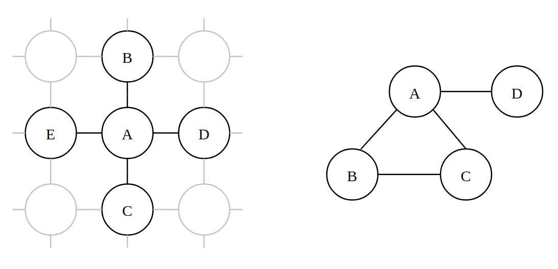
We model a set of random variables $\mathbf{X}$ (in our example, $\{A,B,C,D\}$) whose connections are defined by graph $\mathcal{G}$ and have “potential functions” defined on each of its maximal cliques $\mathcal{Q}\in \mathrm{Cliques}(\mathcal{G})$. The total potential of the graph is defined as

$$\mathrm{\Phi }(\mathbf{x})=\prod _{\mathcal{Q}\in \mathrm{Cliques}(\mathcal{G})}{\varphi }_{\mathcal{Q}}(q)$$

$q$ is an arbitrary instantiation of the set of RVs denoted by $\mathcal{Q}$. The potential functions ${\varphi }_{\mathcal{Q}}(q)\in {\mathbb{R}}_{>0}$ are basically “affinity” functions on the state space of the cliques, e.g. given a state $q$ of a clique $\mathcal{Q}$, the corresponding potential function ${\varphi }_{\mathcal{Q}}(q)$ returns the viability of that state OR how likely that state is. Potential functions are somewhat analogous to conditional densities from Directed PGMs, except for the fact that potentials are arbitrary non-negative values. They don’t necessarily sum to one. For a concrete example, the example graph in Fig.1(b) can thus be factorized as ${\displaystyle \mathrm{\Phi }(a,b,c,d)={\varphi }_{\{A,B,C\}}(a,b,c)\cdot {\varphi }_{\{A,D\}}(a,d)}$. If we assume the variables $\{A,D\}$ are binary RVs, the potential function corresponding to that clique, at its simplest, could be a table like this:

$${\varphi }_{\{A,D\}}(a=0,d=0)=+4.00$$ $${\varphi }_{\{A,D\}}(a=0,d=1)=+0.23$$ $${\varphi }_{\{A,D\}}(a=1,d=0)=+5.00$$ $${\varphi }_{\{A,D\}}(a=1,d=1)=+9.45$$

Just like every other model in machine learning, the potential functions can be parameterized, leading to

$$\begin{array}{}\text{(1)}& \mathrm{\Phi }(\mathbf{x};\mathrm{\Theta })=\prod _{\mathcal{Q}\in \mathrm{Cliques}(\mathcal{G})}{\varphi }_{\mathcal{Q}}(q;{\mathrm{\Theta }}_{\mathcal{Q}})\end{array}$$

Semantically, potentials denotes how likely a given state is. So, higher the potential, more likely that state is.

Reparameterizing in terms of Energy

When we are defining a model, however, it is inconvenient to choose a constrained (non-negative valued) parameterized function. We can easily reparameterize each potential function in terms of energy functions $E_{\mathcal{Q}}$ where

$$\begin{array}{}\text{(2)}& {\varphi }_{\mathcal{Q}}(q,{\mathrm{\Theta }}_{\mathcal{Q}})=\exp (-E_{\mathcal{Q}}(q;{\mathrm{\Theta }}_{\mathcal{Q}}))\end{array}$$

The $\exp (\cdot )$ enforces the potentials to be always non-negative and thus we are free to choose an unconstrained energy function. One question you might ask - “why the negative sign ?”. Frankly, there is no functional purpose of that negative sign. All it does is reverts the semantic meaning of the parameterized function. When we were dealing in terms of potentials, a state which is more likely, had higher potential. Now its opposite - states that are more likely have less energy. Does this semantics sound familiar ? It actually came from Physics where we deal with “energies” (potential, kinetic etc.) which are bad, i.e. less energy means a stable system.

Such reparameterization affects the semantics of Eq.1 as well. Putting Eq.2 into Eq.1 yields

$$\begin{array}{rl}\mathrm{\Phi }(\mathbf{x};\mathrm{\Theta })& =\prod _{\mathcal{Q}\in \mathrm{Cliques}(\mathcal{G})}\exp (-E_{\mathcal{Q}}(q;{\mathrm{\Theta }}_{\mathcal{Q}}))\\ \text{(3)}& & =\exp (-\sum _{\mathcal{Q}\in \mathrm{Cliques}(\mathcal{G})}{E}_{\mathcal{Q}}(q;{\mathrm{\Theta }}_{\mathcal{Q}}))=\exp (-E_{\mathcal{G}}(\mathbf{x};\mathrm{\Theta }))\end{array}$$

Here we defined $E_{\mathcal{G}}(\mathbf{x};\mathrm{\Theta })\triangleq \sum _{\mathcal{Q}\in \mathrm{Cliques}(\mathcal{G})}{E}_{\mathcal{Q}}(q;{\mathrm{\Theta }}_{\mathcal{Q}})$ to be the energy of the whole model. Please note that the reparameterization helped us to convert the relationship between individual cliques and whole graph from multiplicative (Eq.1) to additive (Eq.3). This implies that when we design energy functions for such undirected models, we design energy functions for each individual cliques and just add them.

All this is fine .. well .. unless we need to do things like sampling, computing log-likelihood etc. Then our energy-based parameterization fails because its not easy to incorporate an un-normalized function into probabilistic frameworks. So we need a way to get back to probabilities.

Back to Probabilities

The obvious way to convert un-normalized potentials of the model to normalized distribution is to explicitely normalize Eq.3 over its domain

$$\begin{array}{rl}p(\mathbf{x};\mathrm{\Theta })& =\frac{\mathrm{\Phi }(\mathbf{x};\mathrm{\Theta })}{\sum _{{\mathbf{x}}^{\prime }\in \mathrm{Dom}(\mathbf{X})}\mathrm{\Phi }({\mathbf{x}}^{\prime };\mathrm{\Theta })}\\ \\ \text{(4)}& & =\frac{\exp (-E_{\mathcal{G}}(\mathbf{x};\mathrm{\Theta })/\tau )}{\sum _{{\mathbf{x}}^{\prime }\in \mathrm{Dom}(\mathbf{X})}\exp (-E_{\mathcal{G}}({\mathbf{x}}^{\prime };\mathrm{\Theta })/\tau )}\text{ (using Eq.3)}\end{array}$$

This is the probabilistic model implicitely defined by the enery functions over the whole state-space. [We will discuss $\tau$ shortly. Consider it to be 1 for now]. If the reader is familiar with Statistical Mechanics at all, they might find it extremely similar to Boltzmann Distribution. Here’s what the Wikipedia says:

In statistical mechanics and mathematics, a Boltzmann distribution (also called Gibbs distribution) is a probability distribution or probability measure that gives the probability that a system will be in a certain state as a function of that state’s energy …

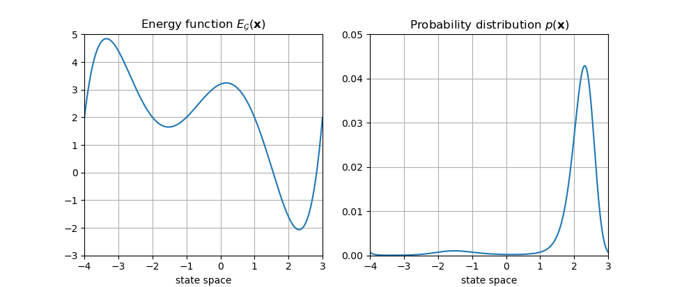
From now on, Eq.4 will be the sole connection between energy-space and probability-space. We can now forget about potential functions. A 1-D example of an energy function and the corresponding probability distribution is shown below:

Fig.2: An energy function and its corresponding probability distribution.

The denominator of Eq.4 is often known as the “Partition Function” (denoted as $Z$). Whatever may be the name, it is quite difficult to compute in general. Because the summation grows exponentially with the space of $\mathbf{X}$.

A hyper-parameter called “temperature” (denoted as $\tau$) is often introduced in Eq.4 which also has its roots in the original Boltzmann Distribution from Physics. A decrease in temperature gathers the probability mass near the lowest energy regions. If not specified, consider $\tau =1$ for the rest of the article.

A general learning algorithm

The question now is - how do I learn the model given a dataset ? Let’s say my dataset has $N$ samples: $\mathcal{D}=\{x^{(i)}{\}}_{i=1}^N$. An obvious way to derive a learning algorithm is to minimize the Negative Log-Likelihood (NLL) loss of the model over our dataset

$$\begin{array}{rl}\mathcal{L}(\mathrm{\Theta };\mathcal{D})=-\log \prod _{i=1}^{N}p(x^{(i)};\mathrm{\Theta })& =\sum _{i=1}^N-\log p(x^{(i)};\mathrm{\Theta })\\ & =\underset{\text{expectation}}{\underbrace{\frac{1}{N}\sum _{i=1}^N}}[E_{\mathcal{G}}(x^{(i)};\mathrm{\Theta })]+\log Z\\ & \text{(putting Eq.4 followed by trivial calculations, and}\\ & \text{ dividing loss by constant N doesn’t affect optima)}\\ \\ & ={\mathbb{E}}_{x\sim p_{\mathcal{D}}}[E_{\mathcal{G}}(x;\mathrm{\Theta })]+\log Z\end{array}$$

Computing gradient w.r.t. parameters yields

$$\begin{array}{rl}\frac{\partial \mathcal{L}}{\partial \mathrm{\Theta }}& ={\mathbb{E}}_{x\sim p_{\mathcal{D}}}\left[\frac{\partial E_{\mathcal{G}}}{\partial \mathrm{\Theta }}\right]+\frac{\partial }{\partial \mathrm{\Theta }}\log Z\\ & ={\mathbb{E}}_{x\sim p_{\mathcal{D}}}\left[\frac{\partial E_{\mathcal{G}}}{\partial \mathrm{\Theta }}\right]+\frac{1}{Z}\frac{\partial }{\partial \mathrm{\Theta }}[\sum _{{\mathbf{x}}^{\prime }\in \mathrm{Dom}(\mathbf{X})}\exp (-E_{\mathcal{G}})]\text{ (using definition of Z)}\\ \\ & ={\mathbb{E}}_{x\sim p_{\mathcal{D}}}\left[\frac{\partial E_{\mathcal{G}}}{\partial \mathrm{\Theta }}\right]+\sum _{{\mathbf{x}}^{\prime }\in \mathrm{Dom}(\mathbf{X})}\underset{\text{RHS of Eq.4}}{\underbrace{\frac{1}{Z}\exp (-E_{\mathcal{G}})}}\cdot \frac{\partial (-E_{\mathcal{G}})}{\partial \mathrm{\Theta }}\\ & \text{ (Both Z and the partial operator are independent}\\ & \text{ of x and can be pushed inside the summation)}\\ \\ & ={\mathbb{E}}_{x\sim p_{\mathcal{D}}}\left[\frac{\partial E_{\mathcal{G}}}{\partial \mathrm{\Theta }}\right]-\underset{\text{expectation}}{\underbrace{\sum _{{\mathbf{x}}^{\prime }\in \mathrm{Dom}(\mathbf{X})}p({\mathbf{x}}^{\prime };\mathrm{\Theta })}}\cdot \frac{\partial E_{\mathcal{G}}}{\partial \mathrm{\Theta }}\\ \text{(5)}& & ={\mathbb{E}}_{x\sim p_{\mathcal{D}}}\left[\frac{\partial E_{\mathcal{G}}}{\partial \mathrm{\Theta }}\right]-{\mathbb{E}}_{x\sim {\mathcal{p}}_{\mathcal{\Theta }}}\left[\frac{\partial E_{\mathcal{G}}}{\partial \mathrm{\Theta }}\right]\end{array}$$

Take a few minutes to digest Eq.5. That’s a very important result. It would be worth discussing it a bit further. The first term in Eq.5 is often known as the “Positive Phase” and the second term as “Negative Phase”. The only difference between them, as you can see, is in the distributions on which the expectations are taken. The first expectation is on the data distribution - essentially picking up data from our dataset. The second expectation is on the model distribution - sampling from the model with current parameters. To understand their semantic interpretation, we need to see them in isolation. For the sake of explanation, consider both terms separately yielding a parameter update rule

$$\mathrm{\Theta }:=\mathrm{\Theta }-\lambda \cdot {\mathbb{E}}_{x\sim \mathcal{D}}\left[\frac{\partial E_{\mathcal{G}}}{\partial \mathrm{\Theta }}\right]\text{, and }\mathrm{\Theta }:=\mathrm{\Theta }+\lambda \cdot {\mathbb{E}}_{x\sim {\mathcal{p}}_{\mathcal{\Theta }}}\left[\frac{\partial E_{\mathcal{G}}}{\partial \mathrm{\Theta }}\right]$$

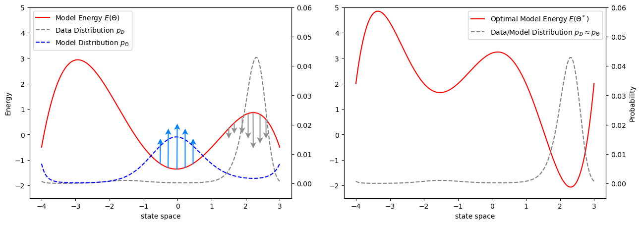
The first update rule basically tries to changes the parameters in a way it can minimize the enrgy function at points coming from data. And the second one tries to maximize (notice the difference in sign) the energy function at points coming from the model. The original update rule (combining both of them) have both of these effects working simulteneously. The minima of the loss landscape occurs when our model discovers the data distribution, i.e. $p_{\mathrm{\Theta }}\approx p_{\mathcal{D}}$. At this point, both positive and negative phase is approximately same and the gradient becomes zero (i.e., no more progress). Below is a clear picture of the update process. The algorithm pushes the energy down at places where original data lies; it also pull the energy up at places which the model thinks original data lies.

Fig.3: (a) Model is being optimized. The arrows depict the “pulling up” and “pushing down” of energy landscape. (b) Model has converged to an optimum.

Whatever may be the interpretation, as I mentioned before that the denominator of $p(\mathbf{x};\mathrm{\Theta })$ (see Eq.4) is intractable in general case, computing the expectation in negative phase is extremely hard. In fact, that is the only difficulty that makes this algorithm practically challenging.

Gibbs Sampling

As we saw in the last section, the only difficulty we have in implementing Eq.5 is not being able to sample from an intractable density (Eq.4). It tuns out, however, that the conditional densities of a small subset of variables given the others is indeed tractable in most cases. That is because, for conditionals, the $Z$ cancels out. Conditional density of one variable (say $X_j$) given the others (let’s denote by $X_{-j}$) is:

$$\begin{array}{}\text{(6)}& p(x_j|{\mathbf{x}}_{-j})=\frac{p(\mathbf{x})}{p({\mathbf{x}}_{-j})}=\frac{\exp (-E_{\mathcal{G}}(\mathbf{x}))}{\sum _{x_j}\exp (-E_{\mathcal{G}}(\mathbf{x}))}\text{ (using Eq.4)}\end{array}$$

I excluded the parameter symbols for notational brevity. That summation in denominator is not as scary as the one in Eq.4 - its only on one variable. We take advantage of this and wisely choose a sampling algorithms that uses conditional densities. Its called Gibbs Sampling. Well, I am not going to prove it. You either have to take my words OR read about it in the link provided. For the sake of this article, just believe that the following works.

To sample $\mathbf{x}\sim p_{\mathrm{\Theta }}(\mathbf{x})$, we iteratively execute the following for $T$ iterations

1. We have a sample from last iteration $t-1$ as ${\mathbf{x}}^{(t-1)}$
2. We then pick one variable $X_j$ (in some order) at a time and sample from its conditional given the others: $x_j^{(t)}\sim p(x_j|\underset{\text{current iteration}}{\underbrace{x_1^{(t)},\cdots ,x_{j-1}^{(t)}}},\underset{\text{previous iteration}}{\underbrace{x_{j+1}^{(t-1)},\cdots ,x_D^{(t-1)}}})$. Please note that once we sampled one variable, we fix its value to the latest, otherwise we keep the value from previous iteration.

We can start this process by setting ${\mathbf{x}}^{(0)}$ to anything. If $T$ is sufficiently large, the samples towards the end are true samples from the density $p_{\mathrm{\Theta }}$. To know it a bit more rigorously, I highly recommend to go through this. You might be curious as to why this algorithm has an iterative process. Thats because Gibbs sampling is an MCMC family algorithm which has something called “Burn-in period”.

Now that we have pretty much everything needed, let’s explore some popular model based on the general principles of EBMs.

Boltzmann Machine

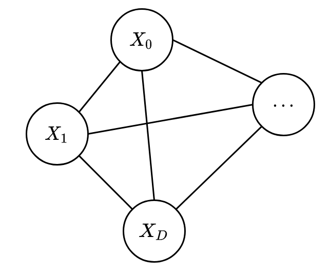
Boltzmann Machine (BM) is one particular model that has been in the literature for a long time. BM is the simplest one in its family and is used for modelling a binary random vector $\mathbf{X}\in \{0,1{\}}^D$ with $D$ components $[X_1,X_2,\cdots ,X_D]$. All $D$ RVs are connected to all others by an undirected graph $\mathcal{G}$.

Fig.4: Undirected graph representing Boltzmann Machine

By design, BM has a fully connected graph and hence only one maximal clique (containing all RVs). The energy function used in BM is possibly the simplest one you can imagine:

$$\begin{array}{}\text{(7)}& E_{\mathcal{G}}(\mathbf{x};W)=-\frac{1}{2}{\mathbf{x}}^{T}W\mathbf{x}\end{array}$$

Upon expanding the vectorized form (reader is encouraged to try), we can see each term $x_i\cdot W_{ij}\cdot x_j$ for all $i<j$ as the contribution of pair of RVs $(X_i,X_j)$ to the whole energy function. $W_{ij}$ is the “connection strength” between them. If a pair of RVs $(X_i,X_j)$ turn on together more often, a high value of $W_{ij}$ would encourage reducing the total energy. So by means of learning, we expect to see $W_{ij}$ going up if $(X_i,X_j)$ fire together. This phenomenon is the founding idea of a closely related learning strategy called Hebbian Learning, proposed by Donald Hebb. Hebbian theory basically says:

If fire together, then wire together

How do we learn this model then ? We have already seen the general way of computing gradient. We have ${\displaystyle \frac{\partial E_{\mathcal{G}}}{\partial W}=-\mathbf{x}{\mathbf{x}}^T}$. So let’s use Eq.5 to derive a learning rule:

$$W:=W-\lambda \cdot ({\mathbb{E}}_{\mathbf{x}\sim p_{\mathcal{D}}}[-\mathbf{x}{\mathbf{x}}^T]-{\mathbb{E}}_{\mathbf{x}\sim \mathrm{Gibbs}(p_W)}[-\mathbf{x}{\mathbf{x}}^T])$$

Equipped with Gibbs sampling, it is pretty easy to implement now. But my description of the Gibbs sampling algorithm was very general. We have to specialize it for implementing BM. Remember that conditional density we talked about (Eq.6) ? For the specific energy function of BM (Eq.7), that has a very convenient and tractable form:

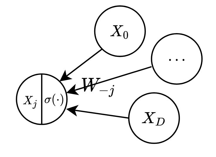
$$p(x_j=1|{\mathbf{x}}_{-j};W)=\sigma (W_{-j}^T\cdot {\mathbf{x}}_{-j})$$

where $\sigma (\cdot )$ is the Sigmoid function and $W_{-j}\in {\mathbb{R}}^{D-1}$ denote the vector of parameters connecting $x_j$ with the rest of the variables ${\mathbf{x}}_{-j}\in {\mathbb{R}}^{D-1}$. I am leaving the proof for the readers; its not hard, maybe a bit lengthy [Hint: Just put the BM energy function in Eq.6 and keep simplifying]. This particular form makes the nodes behave somewhat like computation units (i.e., neurons) as shown in Fig.5 below:

Fig.5: The computational view of BM showing its dependencies by arrows.

Boltzmann Machine with latent variables

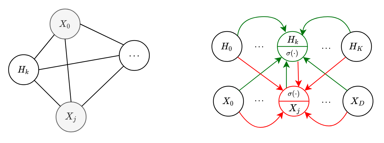
To add more expressiveness in the model, we can introduce latent/hidden variables. They are not observed, but help explaining the visible variables (see my Directed PGM article). However, all variables are still fully connected to each other (shown below in Fig.6(a)).

[ A little disclaimer that as we have already covered a lots of founding ideas, I am going to go over this a bit faster. You may have to look back and find analogies with our previous formulations ]

Fig.6: (a) Undirected graph of BM with hidden units (shaded ones are visible). (b) Computational view of the model while computing conditionals.

Suppose we have $K$ hidden units and $D$ visible ones. The energy function is defined very similar to that of normal BM. Now it contains seperate terms for visible-hidden ($W\in {\mathbb{R}}^{D\times K}$), visible-visible ($V\in {\mathbb{R}}^{D\times D}$) and hidden-hidden ($U\in {\mathbb{R}}^{K\times K}$) interactions. We compactly represent them as $\mathrm{\Theta }\triangleq \{W,U,V\}$.

$$E_{\mathcal{G}}(\mathbf{x},\mathbf{h};\mathrm{\Theta })=-{\mathbf{x}}^{T}W\mathbf{h}-\frac{1}{2}{\mathbf{x}}^{T}V\mathbf{x}-\frac{1}{2}{\mathbf{h}}^{T}U\mathbf{h}$$

The motivation for such energy function is very similar to original BM. However, our probabilistic form of the model is no longer Eq.4, but the marginalized joint distribution.

$$p(\mathbf{x};\mathrm{\Theta })=\sum _{\mathbf{h}\in \mathrm{Dom}(\mathbf{H})}p(\mathbf{x},\mathbf{h};\mathrm{\Theta })=\sum _{\mathbf{h}\in \mathrm{Dom}(\mathbf{H})}\frac{\exp (-E_{\mathcal{G}}(\mathbf{x},\mathbf{h}))}{\sum _{{\mathbf{x}}^{\prime },{\mathbf{h}}^{\prime }\in \mathrm{Dom}(\mathbf{X},\mathbf{H})}\exp (-E_{\mathcal{G}}({\mathbf{x}}^{\prime },{\mathbf{h}}^{\prime }))}$$

It might look a bit scary, but its just marginalized over the hidden state-space. Very surprisingly though, the conditionals have pretty similar forms as original BM:

$$\begin{array}{r}p(h_k|\mathbf{x},{\mathbf{h}}_{-k})=\sigma (W\cdot \mathbf{x}+U_{-k}\cdot {\mathbf{h}}_{-k})\\ p(x_j|\mathbf{h},{\mathbf{x}}_{-j})=\sigma (W\cdot \mathbf{h}+V_{-j}\cdot {\mathbf{x}}_{-j})\end{array}$$

Hopefully the notations are clear. If they are not, try comparing with the ones we used before. I recommend the reader to try proving it as an exercise. The diagram in Fig.6(b) hopefully adds a bit more clarity. It shows a similar computation graph for the conditionals we saw before in Fig.5.

Coming to the gradients, they also takes similar forms as original BM .. only difference is that now we have more parameters

$$\begin{array}{rl}W& :=W-\lambda \cdot ({\mathbb{E}}_{\mathbf{x}\mathbf{,}\mathbf{h}\sim p_{\mathcal{D}}}[-\mathbf{x}{\mathbf{h}}^T]-{\mathbb{E}}_{\mathbf{x}\mathbf{,}\mathbf{h}\sim \mathrm{Gibbs}(p_{\mathrm{\Theta }})}[-\mathbf{x}{\mathbf{h}}^T])\\ V& :=V-\lambda \cdot ({\mathbb{E}}_{\mathbf{x}\sim p_{\mathcal{D}}}[-\mathbf{x}{\mathbf{x}}^T]-{\mathbb{E}}_{\mathbf{x}\sim \mathrm{Gibbs}(p_{\mathrm{\Theta }})}[-\mathbf{x}{\mathbf{x}}^T])\\ U& :=U-\lambda \cdot ({\mathbb{E}}_{\mathbf{h}\sim p_{\mathcal{D}}}[-\mathbf{h}{\mathbf{h}}^T]-{\mathbb{E}}_{\mathbf{h}\sim \mathrm{Gibbs}(p_{\mathrm{\Theta }})}[-\mathbf{h}{\mathbf{h}}^T])\end{array}$$

If you are paying attention, you might notice something strange .. how do we compute the terms ${\mathbb{E}}_{\mathbf{h}\sim p_{\mathcal{D}}}$ (in the positive phase) ? We don’t have hidden vectors in our dataset, right ? Actually, we do have visible vectors ${\mathbf{x}}^{(i)}$ in dataset and we can get an approximate complete data (visible plus hidden) density as

$$p_{\mathcal{D}}({\mathbf{x}}^{(i)},\mathbf{h})=p_{\mathcal{D}}({\mathbf{x}}^{(i)})\cdot p_{\mathrm{\Theta }}(\mathbf{h}|{\mathbf{x}}^{(i)})$$

Basically, we sample a visible data from our dataset and use the conditional to sample a hidden vector. We fix the visible vector and them sample from the hidden vector one component at a time (using Gibbs sampling).

For jointly sampling a visible and hidden vector from the model (for negative phase), we also use Gibbs sampling just as before. We sample all of visible and hidden RVs component by component starting the iteration from any random values. There is a clever hack though. What we can do is we can start the Gibbs iteration by fixing the visible vector to a real data from our dataset (and not anything random). Turns out, this is extremely useful and efficient for getting samples quickly from the model distribution. This algorithm is famously known as “Contrastive Divergence” and has long been used in practical implementations.

“Restricted” Boltzmann Machine (RBM)

Here comes the all important RBM, which is probably one of the most famous energy based models of all time. But, guess what, I am not going to describe it bit by bit. We have already covered enough that we can quickly build on top of them.

RBM is basically same as Boltzmann Machine with hidden units but with one big difference - it doesn’t have visible-visible AND hidden-hidden interactions, i.e.

$$U=\mathbf{0},V=\mathbf{0}$$

If you do just that, Boooom ! You get RBMs (see its graphical diagram in Fig.7(a)). It makes the formulation much simpler. I am leaving it entirely for the reader to do majority of the math. Just get rid of $U$ and $V$ from all our formulations in last section and you are done. Fig.7(b) shows the computational view of RBM while computing conditionals.

Fig.7: (a) Graphical diagram of RBM. (b) Arrows just show computation deps

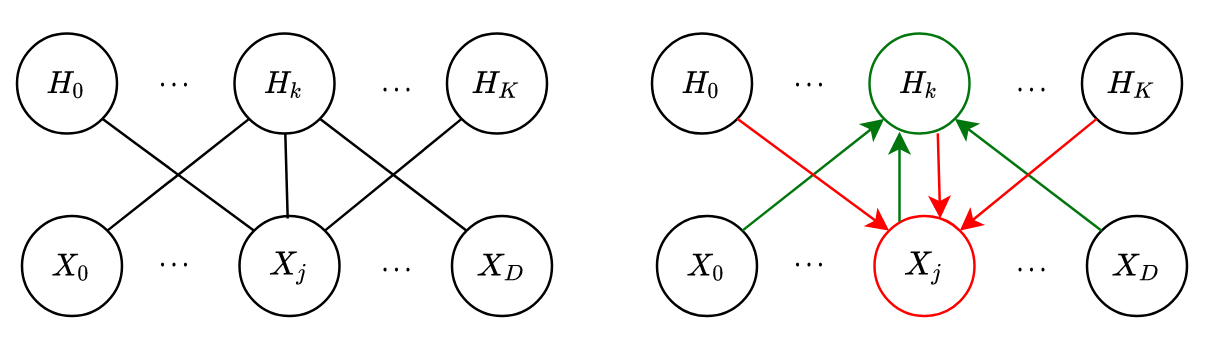
Let me point you out one nice consequence of this model: the conditionals for each visible node is independent of the other visible nodes and this is true for hidden nodes as well.

$$\begin{array}{r}p(h_k|\mathbf{x})=\sigma (W_{[:,k]}\cdot \mathbf{x})\\ p(x_j|\mathbf{h})=\sigma (W_{[j,:]}\cdot \mathbf{h})\end{array}$$

That means they can be computed in parallel

$$\begin{array}{r}p(\mathbf{h}|\mathbf{x})=\prod _{k=1}^{K}p(h_k|\mathbf{x})=\sigma (W\cdot \mathbf{x})\\ p(\mathbf{x}|\mathbf{h})=\prod _{j=i}^{D}p(x_j|\mathbf{h})=\sigma (W\cdot \mathbf{h})\end{array}$$

Moreover, the Gibbs sampling steps become super easy to compute. We just have to iterate the following steps:

1. Sample a hidden vector ${\mathbf{h}}^{(t)}\sim p(\mathbf{h}|{\mathbf{x}}^{(t-1)})$
2. Sample a visible vector ${\mathbf{x}}^{(t)}\sim p(\mathbf{x}|{\mathbf{h}}^{(t)})$

This makes RBM an attractive choice for practical implementation.

---

Whoahh ! That was a heck of an article. I encourage everyone to try working out the RBM math more rigorously by themselves and also implement it in a familiar framework. Alright, that’s all for this article.

References

1. Boltzmann Machine, by G. Hinton, 2007
2. Notes on Boltzmann Machine, by Patrick Kenny
3. deeplearning.net documentation
4. Hinton’s coursera course
5. Deep Learning Book by Ian Goodfellow, Yoshua Bengio and Aaron Courville