Neural Ordinary Differential Equation (Neural ODE)

Neural Ordinary Differential Equation (Neural ODE) is a very recent and first-of-its-kind idea that emerged in NeurIPS 2018. The authors, four researchers from University of Toronto, reformulated the parameterization of deep networks with differential equations, particularly first-order ODEs. The idea evolved from the fact that ResNet, a very popular deep network, possesses quite a bit of similarity with ODEs in their core structure. The paper also offered an efficient algorithm to train such ODE structures as a part of a larger computation graph. The architecture is flexible and memory efficient for learning. Being a bit non-trivial from a deep network standpoint, I decided to dedicate this article explaining it in detail, making it easier for everyone to understand. Understanding the whole algorithm requires fair bit of rigorous mathematics, specially ODEs and their algebric understanding, which I will try to cover at the beginning of the article. I also provided a (simplified) PyTorch implementation that is easy to follow.

Ordinary Differential Equations (ODE)

Definition

Let’s put Neural ODEs aside for a moment and take a refresher on ODE itself. Because of their unpopularity in the deep learning community, chances are that you haven’t looked at them since high school. We will focus our discussion on first-order linear ODEs which takes a generic form of

$$\frac{dx}{dt}=f(x,t)$$

where ${\displaystyle x,t,\frac{dx}{dt}\in \mathbb{R}}$. Please recall that ODEs are differential equations that involve only one independent variable, which in our case is $t$. Geometrically, such an ODE represents a family of curves/functions $x(t)$, also called the solutions of the ODE. The function $f(x,t)$, often called the dynamics of the system, denotes a common characteristics of all the solutions. Specifically, it denotes the first-derivative (slope) of all the solutions. An example would make things clear: let’s say the dynamics of an ODE is ${\displaystyle f(x,t)=2xt}$. With the help of basic calculus, we can see the family of solutions are ${\displaystyle x(t)=k\cdot e^{t^2}}$ for any value of $k$.

System of ODEs

Just like any other algorithms in Deep Learning, we can (and we have to) go beyond $\mathbb{R}$ space and eshtablish similar ODEs in higher dimension. A system of ODEs with dependent variables $x_1,x_2,\cdots x_d\in \mathbb{R}$ and independent variable $t\in \mathbb{R}$ can be written as

$$\frac{d{x}_1}{dt}=f_1(x_1,x_2,\cdots ,x_d,t);\frac{d{x}_2}{dt}=f_2(x_1,x_2,\cdots ,x_d,t);\cdots$$

With a vectorized notation of $\mathbf{x}\triangleq [x_1,x_2,\cdots ,x_d{]}^T\in {\mathbb{R}}^d$ and $\mathbf{f}(\mathbf{x})\triangleq [f_1,f_2,\cdots ,f_d{]}^T\in {\mathbb{R}}^d$, we can write

$$\frac{d\mathbf{x}}{dt}=\mathbf{f}(\mathbf{x},t)$$

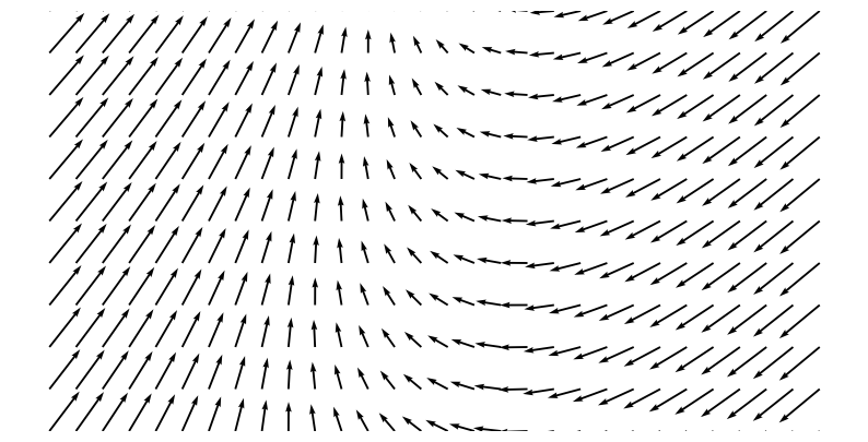
The dynamics $\mathbf{f}(\mathbf{x},t)$ can be seen as a Vector Field where given any $\mathbf{x}\in {\mathbb{R}}^d$, $\mathbf{f}\in {\mathbb{R}}^d$ denotes its gradient with respect to $t$. The independent variable $t$ can often be regarded as time. For example, Fig.1 shows the ${\mathbb{R}}^2$ space and a dynamics $\mathbf{f}(\mathbf{x},t)=tanh(W\mathbf{x}+b)$ defined on it. Please note that it is a time-invariant system, i.e., the dynamics is independent of $t$. A system with time-dependent dynamics would have a different gradient on a given $\mathbf{x}$ depending on which time you visit it.

Fig.1: A vector field in 2D space denoting the dynamics of an ODE

Initial Value Problem

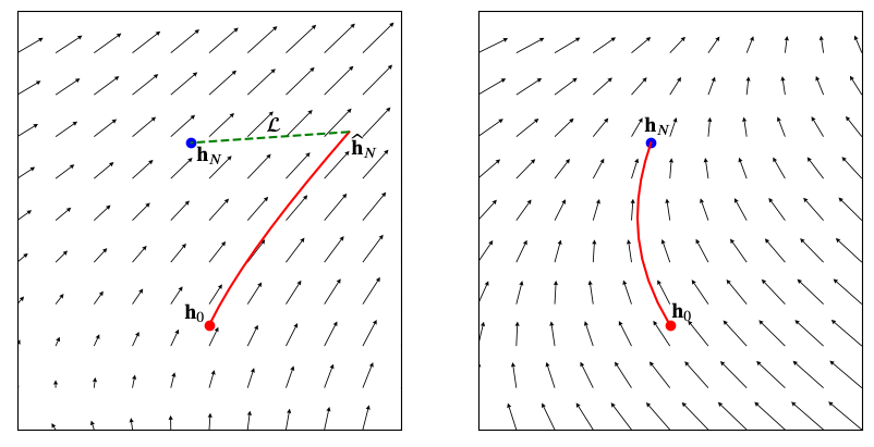
Although I showed the solution of an extremely simple system with dynamics $f(x,t)=2xt$, most practical systems are far from it. Systems with higher dimension and complicated dynamics are very difficult to solve analytically. This is when we resort to numerical methods. A specific way of solving any ODE numerically is to solve an Initial Value Problem where given the system (dynamics) and an initial condition, one can iteratively “trace” the solution. I emphasized the term trace because that’s what it is. Think of it as dropping a small particle on the vector field at some point and let it flow according to the gradients at any point.

Fig.2: Solving for two solutions with two different initial condition

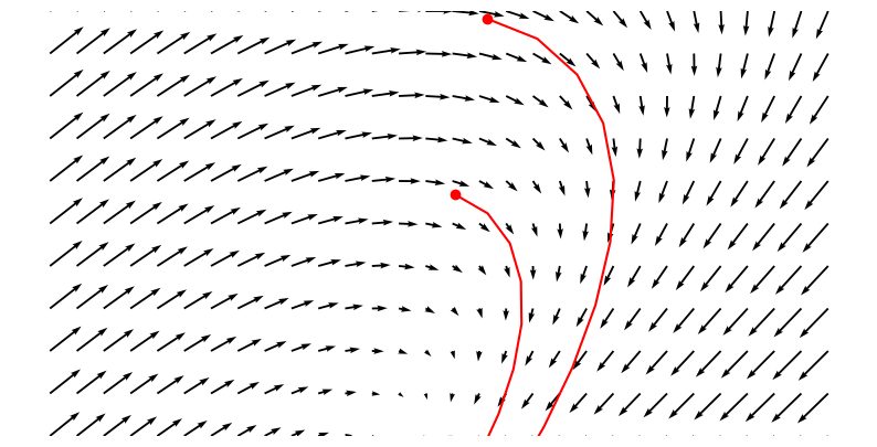
Fig.2 shows two different initial condition (red dots) leads to two different curves/solution (a small segment of the curve is shown). These curves/solutions are from the family of curves represented by the system whose dynamics is shown with black arrows. Different numerical methods are available on how well we do the “tracing” and how much error we tolerate. Strating from naive ones, we have modern numerical solvers to tackle the initial value problems. We will focus on one of the simplest yet popular method known as Forward Eular’s method for the sake of simplicity. The algorithm simply does the following: It starts from a given initial state ${\mathbf{x}}_0$ at $t=0$ and literally goes in the direction of gradient at that point, i.e. $\mathbf{f}(\mathbf{x}={\mathbf{x}}_0,t=0)$ and keeps doing it till $t=N$ using a small step size of $\mathrm{\Delta }t\triangleq t_{i+1}-t_i$. The following iterative update rule summerizes everything

$${\mathbf{x}}_{t+1}={\mathbf{x}}_t+\mathrm{\Delta }t\cdot \mathbf{f}({\mathbf{x}}_t,t)$$

In case you haven’t noticed, the formula can be obtained trivially from the discretized version of analytic derivative

$$\mathbf{f}(\mathbf{x},t)=\frac{d\mathbf{x}}{dt}\approx \frac{{\mathbf{x}}_{t+1}-{\mathbf{x}}_t}{\mathrm{\Delta }t}$$

If you look at Fig.2 closely enough, you would see the red curves are made up of discrete segements which is a result of solving an initial value problem using Forward Eular’s method.

Motivation of Neural ODE

Let’s look at the core structure of ResNet, an extremely popular deep network that almost revolutionized deep network architecture. The most unique structural component of ResNet is its residual blocks that computes “increaments” on top of previous layer’s activation instead of activations directly. If the activation of layer $t$ is ${\mathbf{h}}_t$ then

$$\begin{array}{}\text{(1)}& {\mathbf{h}}_{t+1}={\mathbf{h}}_t+\mathbf{F}({\mathbf{h}}_t;{\theta }_t)\end{array}$$

where $\mathbf{F}(\cdot )$ is the residual function (increament on top of last layer). I am pretty sure the reader can feel where it’s going. Yes, the residual architectire resembles the forward eular’s method on an ODE with dynamics $\mathbf{F}(\cdot )$. Having $N$ such residual layers is similar to executing $N$ steps of forward eular’s method with step size $\mathrm{\Delta }t=1$. The idea of Neural ODE is to “parameterize the dynamics of this ODE explicitely rather than parameterizing every layer”. So we can have

$$\frac{d{\mathbf{h}}_t}{dt}=\mathbf{F}({\mathbf{h}}_t,t;\theta )$$

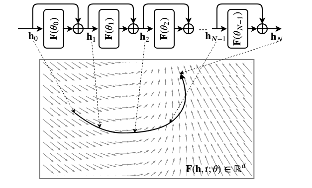
and $N$ successive layers can be realized by $N$-step forward eular evaluations. As you can guess, we can choose $N$ as per our requirement and in limiting case we can think of it as an infinite layer ($N $) network. Although you must understand that such parameterization cannot provide an infinite capacity as the number of parameters is shared and finite. Fig.3 below depicts the resemblance of ResNet with forward eular iteration.

Fig.3: Resemblence of ResNet and Forward Eular’s method.

Parameterization and Forward pass

Although we already went over this in the last section, but let me put it more formally one more time. An “ODE Layer” is basically characterized by its dynamics function $\mathbf{F}({\mathbf{h}}_t,t;\theta )$ which can be realized by a (deep) neural network. This network takes input the “current state” ${\mathbf{h}}_t$ (basically activation) and time $t$ and produces the “direction” (i.e., ${\displaystyle \mathbf{F}({\mathbf{h}}_t,t;\theta )=\frac{d{\mathbf{h}}_t}{dt}}$) where the state should go next. A full forward pass through this layer is essentially executing an $N$ step Forward Eular on the ODE with an “initial state” (aka “input”) ${\mathbf{h}}_0$. $N$ is a hyperparameter we choose and can be compared to “depth” in standard deep neural network. Following the original paper’s convention (with a bit of python-style syntax), we write the forward pass as

$$\begin{array}{}\text{(2)}& {\mathbf{h}}_N=\mathrm{ODESolve}(start\mathrm{\_}state={\mathbf{h}}_0,dynamics=\mathbf{F},t\mathrm{\_}start=0,t\mathrm{\_}end=N;\theta )\end{array}$$

where the “ODESolve” is any iterative ODE solver algorithm and not just Forward Eular. By the end of this article you’ll understand why the specific machinery of Eular’s method is not essential.

Coming to the backward pass, a naive solution you might be tempted to offer is to back-propagate thorugh the operations of the solver. I mean, look at the iterative update equation Eq.1 of an ODE Solver (for now just Forward Eular) - everything is indeed differentiable ! But then, it is no better than ResNet, not from a memory cost point of view. Note that backpropagating through a ResNet (and so with any standard deep network) requires storing the intermediate activations to be used later for the backward pass. Such operation is resposible for the memory complexity of backpropagation being linear in number of layers (i.e., $\mathcal{O}(L)$). This is where the authors proposed a brilliant idea to make it $\mathcal{O}(1)$ by not storing the intermediate states.

Fig.3: Block diagram of ODE Layer.

“Adjoint method” and the backward pass

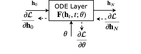
Just like any other computational graph associated with a deep network, we get a gradient signal coming from the loss. Let’s denote the incoming gradient at the end of the ODE layer as ${\displaystyle \frac{d\mathcal{L}}{d{\mathbf{h}}_N}}$, where $\mathcal{L}$ is a scalar loss. All we have to do is use this incoming gradient to compute ${\displaystyle \frac{d\mathcal{L}}{d\theta }}$ and perform an SGD (or any variant) step. A bunch of parameter updates in the right direction would cause the dynamics to change and consequently the whole trajectory (i.e., trace) except the input. Fig.4 shows a graphical representation of the same. Please note that for simplicity, the loss has been calculated using ${\mathbf{h}}_N$ itself. To be specific, the loss (green dotted line) is the euclidian distance between ${\mathbf{h}}_N$ and its (avaialble) ground truth ${\hat{\mathbf{h}}}_N$.

Fig.4: Effect of updating parameters of the dynamics.

In order to accomplish our goal of computing the parameter gradients, we define a quantity ${\mathbf{a}}_t$, called the “Adjoint state”

$${\mathbf{a}}_t\triangleq \frac{d\mathcal{L}}{d{\mathbf{h}}_t}$$

comparing to a standard neural network, this is basically the gradient of the loss $\mathcal{L}$ w.r.t all intermediate activations (states of the ODE). It is indeed a generalization of a quantity I mentioned earlier, i.e., the incoming gradient into the layer ${\displaystyle \frac{d\mathcal{L}}{d{\mathbf{h}}_N}={\mathbf{a}}_N}$. Although we cannot compute this quantity independently for every timestep, a bit of rigorous mathematics (refer to appendix B.1 of original paper) can show that the adjoint state follows a differential equation with a dynamics function

$$\begin{array}{}\text{(3)}& {\mathbf{F}}_a({\mathbf{a}}_t,{\mathbf{h}}_t,t,\theta )\triangleq \frac{d{\mathbf{a}}_t}{dt}=-{\mathbf{a}}_t\frac{\partial \mathbf{F}}{\partial {\mathbf{h}}_t}\end{array}$$

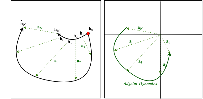
and that’s a good news ! We now have the dynamics that ${\mathbf{a}}_t$ follows and an initial value ${\mathbf{a}}_N$ (value at the extreme end $t=N$). That means we can run an ODE solver backward in time from $t=N\to 0$ and calculate all ${\mathbf{a}}_t$ in succession, like this

$${\mathbf{a}}_{N-1},\cdots ,{\mathbf{a}}_0=\mathrm{ODESolve}({\mathbf{a}}_N,{\mathbf{F}}_a,N,0;\theta )$$

Please look at Eq.2 for the signature of the “ODESolve” function. This time we also produced all intermediate states of the solver as output. An intuitive visualization of the adjoint state and its dynamics is given in Fig.5 below.

Fig.5: An intuitive visualization of the adjoint state and its dynamics.

The quantity on the right hand side of Eq.3 is a vector-jacobian product where ${\displaystyle \frac{\partial \mathbf{F}}{\partial {\mathbf{h}}_t}}$ is the jacobian matrix. Given the functional form of $\mathbf{F}$, this can be readily computed using the current state ${\mathbf{h}}_t$ and the latest parameter value. But wait a minute ! I said before that we are not storing the intermediate ${\mathbf{h}}_t$ values. Where do we get them now ? The answer is - we can compute them again. Please remeber that we still have $\mathbf{F}$ with us along with an extreme value ${\mathbf{h}}_N$ (output of the forward pass). We can run another ODE backwards in time starting from $t=N\to 0$. Essentially we can fuse two ODEs together

$$[{\mathbf{a}}_{N-1};{\mathbf{h}}_{N-1}],\cdots ,[{\mathbf{a}}_0;{\mathbf{h}}_0]=\mathrm{ODESolve}([{\mathbf{a}}_N;{\mathbf{h}}_N],[{\mathbf{F}}_a;\mathbf{F}],N,0;\theta )$$

Its basically executing two update equations for two ODEs in one “for loop” traversing from $N\to 0$. The intermediate values of ${\mathbf{h}}_t$ wouldn’t be exactly same as what we got in the forward pass (because no numerical solver is of infinite precision), but they are indeed good approximations.

Okay, what about the parameters of the model (dynamics) ? How do we get to our ultimate goal, ${\displaystyle \frac{d\mathcal{L}}{d\theta }}$ ?

Let’s define another quantity very similar to the adjoint state, i.e., the parameter gradient of the loss at every step of the ODE solver

$${\mathbf{a}}_t^{\theta }\triangleq \frac{d\mathcal{L}}{d{\theta }_t}$$

Point to note here is that ${\theta }_t=\theta$ as the parameters do not change during a trajectory. Instead, these quantities signify local influences of the parameters at each step of computation. This is very similar to a roll-out of RNN in time where parameters are shared accross time steps. With a proof very similar to that of the adjoint state, it can be shown that

$${\mathbf{a}}_t^{\theta }={\mathbf{a}}_t\frac{\partial \mathbf{F}}{\partial \theta }$$

just like shared-weight RNNs, we can compute the full parameter gradient as combination of local influences

$$\begin{array}{}\text{(4)}& \frac{d\mathcal{L}}{d\theta }={\int }_0^N{\mathbf{a}}_t^{\theta }dt={\int }_0^N{\mathbf{a}}_t\frac{\partial \mathbf{F}}{\partial \theta }dt\end{array}$$

The quantity ${\displaystyle {\mathbf{a}}_t\frac{\partial \mathbf{F}}{\partial \theta }}$ is another vector-jacobian product and can be evaluted using the values of ${\mathbf{h}}_t$, ${\mathbf{a}}_t$ and latest parameter $\theta$. So do we need another pass over the whole trajectory as Eq.4 consists of a integral ? Fortunately, NO. Let me bring your attention to the fact that whatever we need to compute this vector-jacobian is already being computed in the fused ODE we saw before. Furthermore we can tweak the Eq.4 as

$$\begin{array}{}\text{(5)}& \frac{d\mathcal{L}}{d\theta }=\mathbf{0}-{\int }_N^0{\mathbf{a}}_t\frac{\partial \mathbf{F}}{\partial \theta }dt\end{array}$$

I hope you are seeing what I am seeing. This is equivalent to solving yet another ODE (backwards in time, again!) with dynamics ${\displaystyle {\mathbf{F}}_{\theta }({\mathbf{a}}_t,{\mathbf{h}}_t,\theta ,t)\triangleq -{\mathbf{a}}_t\frac{\partial \mathbf{F}}{\partial \theta }}$ and initial state ${\mathbf{a}}_N^{\theta }=\mathbf{0}$. The end state ${\mathbf{a}}_0^{\theta }$ of this ODE completes the whole integral in Eq.5 and therefore is equal to ${\displaystyle \frac{d\mathcal{L}}{d\theta }}$. Just like last time, we can fuse this ODE with the last two combined

$$[{\mathbf{a}}_{N-1};{\mathbf{h}}_{N-1};\mathrm{\_}],\cdots ,[{\mathbf{a}}_0;{\mathbf{h}}_0;{\mathbf{a}}_0^{\theta }]=\mathrm{ODESolve}([{\mathbf{a}}_N;{\mathbf{h}}_N;\mathbf{0}],[{\mathbf{F}}_a;\mathbf{F};{\mathbf{F}}_{\theta }],N,0;\theta )$$

Fig.6: A pictorial representation of the forward and backward pass with all its ODEs.

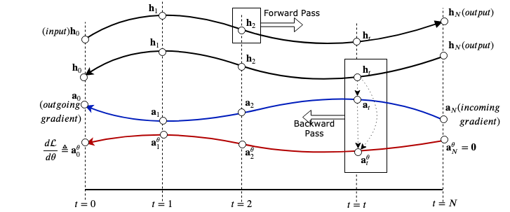
Take some time to digest the final 3-way ODE and make sure you get it. Because that is pretty much it. Once we get the parameter gradient, we can continue with normal stochastic gradient update rule (SGD or family). Additionally you may want to pass ${\mathbf{a}}_0$ to the computation graph that comes before our ODE layer. A representative diagram containing a clear picture of all the ODEs and their interdependencies are shown above.

PyTorch Implementation

Implementing this algorithm is a bit tricky due to its non-conventional approach for gradient computations. Specially if you are using library like PyTorch which adheres to a specific model of computation. I am providing a very simplified implementation of ODE Layer as a PyTorch nn.Module. Because this post has already become quite long and stuffed with maths and new concepts, I am leaving it here. I am putting the core part of the code (well commented) here just for reference but a complete application can be found on this GitHub repo of mine. My implementation is quite simplified as I have hard-coded “Forward Eular” method as the only choice of ODE solver. Feel free to contribute to my repo.

#############################################################
# Full code at https://github.com/dasayan05/neuralode-pytorch
#############################################################

import torch

class ODELayerFunc(torch.autograd.Function):
        
    @staticmethod
    def forward(context, z0, t_range_forward, dynamics, *theta):
        delta_t = t_range_forward[1] - t_range_forward[0] # get the step size
        
        zt = z0.clone()
        for tf in t_range_forward: # Forward eular's method
            f = dynamics(zt, tf)
            zt = zt + delta_t * f # update

        context.save_for_backward(zt, t_range_forward, delta_t, *theta)
        context.dynamics = dynamics # 'save_for_backwards() won't take it, so..
        
        return zt # final evaluation of 'zt', i.e., zT

    @staticmethod
    def backward(context, adj_end):
        # Unpack the stuff saved in forward pass
        zT, t_range_forward, delta_t, *theta = context.saved_tensors
        dynamics = context.dynamics
        t_range_backward = torch.flip(t_range_forward, [0,]) # Time runs backward

        zt = zT.clone().requires_grad_()
        adjoint = adj_end.clone()
        dLdp = [torch.zeros_like(p) for p in theta] # Parameter grads (an accumulator)

        for tb in t_range_backward:
            with torch.set_grad_enabled(True):
                # above 'set_grad_enabled()' is required for the graph to be created ...
                f = dynamics(zt, tb)
                # ... and be able to compute all vector-jacobian products
                adjoint_dynamics, *dldp_ = torch.autograd.grad([-f], [zt, *theta], grad_outputs=[adjoint])
            
            for i, p in enumerate(dldp_):
                dLdp[i] = dLdp[i] - delta_t * p # update param grads
            adjoint = adjoint - delta_t * adjoint_dynamics # update the adjoint
            zt.data = zt.data - delta_t * f.data # Forward eular's (backward in time)

        return (adjoint, None, None, *dLdp)

class ODELayer(torch.nn.Module):

    def __init__(self, dynamics, t_start = 0., t_end = 1., granularity = 25):
        super().__init__()

        self.dynamics = dynamics
        self.t_start, self.t_end, self.granularity = t_start, t_end, granularity
        self.t_range = torch.linspace(self.t_start, self.t_end, self.granularity)

    def forward(self, input):
        return ODELayerFunc.apply(input, self.t_range, self.dynamics, *self.dynamics.parameters())

That’s all for today. See you.