Directed Graphical Models & Variational Inference

Welcome to the first part of a series of tutorials about Directed Probabilistic Graphical Models (PGMs) & Variational methods. Directed PGMs (OR, Bayesian Networks) are very powerful probabilistic modelling techniques in machine learning literature and have been studied rigorously by researchers over the years. Variational Methods are family of algorithms arise in the context of Directed PGMs when it involves solving an intractable integrals. Doing inference on a set of latent variables (given a set of observed variables) involves such an intractable integral. Variational Inference (VI) is a specialised form of variation method that handles this situation. This tutorial is NOT for absolute beginners as I assume the reader to have basic-to-moderate knowledge about Random Variables, probability theories and PGMs. The next tutorial in this series will cover one perticular VI method, namely “Variational Autoencoder (VAE)” built on top of VI.

Fig.1: An example of Directed PGM (Bayesian Network)

A review of Directed PGMs

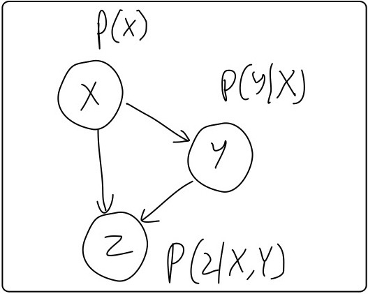
A Directed PGM, also known as Bayesian Network, is a set of random variables (RVs) associated with a graph structure (DAG) expressing conditional independance (CI assumptions) among them. Without the CI assumptions, one had to model the joint distribution over all the RVs, which would’ve been difficult. Fig. 1 shows a typical DAG expressing the conditional independance among the set of participating RVs $\{X,Y,Z\}$. With the CI assumptions in place, we can write the join distribution over $X,Y,Z$ as $$\mathbb{P}(X,Y,Z)=\mathbb{P}(Z|X,Y)\cdot \mathbb{P}(Y|X)\cdot \mathbb{P}(X)$$

In general, joint distribution over a set of RVs $X_1,X_2,\cdots ,X_i,\cdots ,X_N$ with CI assumptions encoded in a graph $\mathbb{G}$ can be written/factorized as

$$\mathbb{P}(X_1,X_2,\cdots ,X_N)=\prod _{i=1}^N\mathbb{P}(X_i|P{a}_{\mathbb{G}}(X_i))$$

Where, $P{a}_{\mathbb{G}}(X_i)$ is the parents of node $X_i$ according to graph $\mathbb{G}$. One can easily verify that the factorization of $\mathbb{P}(X,Y,Z)$ above resembles the general formula.

Ancestral sampling

Fig.2: Ancestral Sampling

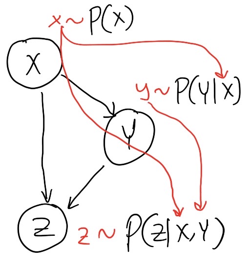
A key idea in Directed PGMs is the way we sample from them. We use something known as Ancestral Sampling. Unlike joint distributions over all random variables ($\mathbb{P}(\cdots ,X_i,\cdots )$), a graph structure (i.e., $\mathbb{G}$) breaks it down into multiple factors which then needs to be synchronized to get a full sample from the graph. Here’s how we do it: 1. We start with RVs with no parent (according to $\mathbb{G}$). We sample from them as usual. 2. Plug the samples in the conditionals involving those RVs. Sample the new RVs from those conditionals. 3. Plug the samples from step 2 further and keep sampling until all variables are sampled.

So, in the example depicted in Fig. 1

$$x\sim \mathbb{P}(X)$$ $$y\sim \mathbb{P}(Y|X=x)$$ $$z\sim \mathbb{P}(Z|Y=y,X=x)$$

So, we get one sample as $(x,y,z)$. In contrast, a full joint distribution needs to be sampled all at once

$$(x,y,z)\sim \mathbb{P}(X,Y,Z)$$

Parameterization and Learning

Now, as we have a clean way of representing a complicated distribution in the form of a graph structure, we can parameterize each individual distribution in the factorized form to parameterize the whole joint distribution. Parameterizing the distribution in the example in Fig. 1

$$\mathbb{P}(Z|X,Y;{\theta }_1)\cdot \mathbb{P}(Y|X;{\theta }_2)\cdot \mathbb{P}(X;{\theta }_3)$$

For convenience, we will write the above factorization as $$p_{model}(X,Y,Z;\theta )$$ where $\theta =\{{\theta }_1,{\theta }_2,{\theta }_3\}$ is the set of all parameters.

For learning, we require a set of data samples (i.e., a dataset) collected from an unknown data generating distribution $p_{data}(X,Y,Z)$. So, a dataset $D=\{x^{(i)},y^{(i)},z^{(i)}{\}}_{i=1}^M$ where each data sample is drawn as

$$x^{(i)},y^{(i)},z^{(i)}\sim p_{data}(X,Y,Z)$$

The likelihood of the data samples under our model signifies the probability that the samples came from our model. It is simply

$$\mathbb{L}(D;\theta )=\prod _{x^{(i)},y^{(i)},z^{(i)}\sim p_{data}}{p}_{model}(x^{(i)},y^{(i)},z^{(i)};\theta )$$

The goal of learning is to get a good estimate of $\theta$. We do it by maximizing the likelihood (or, often log-likelihood) w.r.t $\theta$, which we call Maximum Likelihood Estimation or MLE in short

$$\hat{\theta }=arg\underset{\theta }{max}\log \mathbb{L}(D;\theta )$$

Inference

Inference in a Directed PGM refers to estimating a set of RVs given another set of RVs in a graph $\mathbb{G}$. To do inference, we need to have an already learnt model. Inference is like “answering queries” after gathering knowledge (i.e., learning). For example, in our running example, one may ask, “What is the value of $X$ given $Y=y_0$ and $Z=z_0$ ?”. The question can be answered by constructing the conditional distribution using the definition of conditional probability

$$\mathbb{P}(X|Y=y_0,Z=z_0)=\frac{\mathbb{P}(X,Y=y_0,Z=z_0)}{{\int }_x\mathbb{P}(X,Y=y_0,Z=z_0)}$$

In case a deterministic answer is desired, one can figure out the expected value of $X$ under the above distribution

$$\widehat{x_0}={\mathbb{E}}_{\mathbb{P}(X|Y=y_0,Z=z_0)}[X|Y=y_0,Z=z_0]$$

A generative view of data

Its quite important to understand this point. In this section, I won’t tell you anything new per se, but repeat some of the things I explained in the Ancestral Sampling subsection above.

Given a finite set of data (i.e., a dataset), we start our model building process from asking ourselves one question, “How my data could’ve been generated ?”. The answer to this question is precisely “our model”. The model (i.e., the graph structure) we build is essentially our belief of how the data was generated. Well, we might be wrong. The data may have been generated by some other ways, but we always start with a belief - our model. The reason I started modelling my data with a graph structure shown in Fig.1 is because I believe all my data (i.e, $\{x^{(i)},y^{(i)},z^{(i)}{\}}_{i=1}^M$) was generated as follows:

$$x^{(i)}\sim \mathbb{P}(X)$$ $$y^{(i)}\sim \mathbb{P}(Y|X=x^{(i)})$$ $$z^{(i)}\sim \mathbb{P}(Z|Y=y^{(i)},X=x^{(i)})$$

Or, equivalently

$$(x^{(i)},y^{(i)},z^{(i)})\sim p_{model}(X,Y,Z)$$

Latent variables: A model with “hidden factor”

Equipped with the knowledge of general Directed PGMs, we are now ready to look at one particular model (or rather family of models) that is extremely important and used heavily everywhere in practice. The idea of latent variable is basically our belief of having a hidden factor behind generation of our data. But, the hidden factor is (of course) not available in our dataset. Fig.3 shows the structure of the model (i.e., our belief about the data generation process) which has the variable $Z$ which we believe to be a factor that is latent/hidden, but have contribution in generation of $X$ (i.e., the observed variable). So, my model is as follows:

$$z^{(i)}\sim \mathbb{P}(Z)$$ $$x^{(i)}\sim \mathbb{P}(X|Z=z^{(i)})$$

Or, equivalently

$$(z^{(i)},x^{(i)})\sim p_{model}(X,Z)$$

But unfortunately, the dataset $D=\{x^{(i)}{\}}_i^M$ does not contain $z^{(i)}$

$$x^{(i)}\sim p_{data}(X)$$

An example will clear any doubts:

Fig.3: Latent factor responsible for data generation

Think of our dataset as facial images of $K$ persons, but without identifying them with any labels. So, $D=\{x^{(i)}{\}}_{i=1}^M$ where $x^{(i)}$ is a facial image. But our model may contain a hidden factor, namely, the “identity” of the person in a given image $x^{(i)}$. We can model this with a latent (discrete) variable having $K$ states.

$$\begin{gathered} z^{(i)}\sim \mathbb{P}(Z\in \\ 0,1,\cdots K \\ ) \end{gathered}$$ $$x^{(i)}\sim \mathbb{P}(X|Z=z^{(i)})$$

Let’s see if we can do MLE on this. The likelihood is

$$\mathbb{L}(D;\theta )=\prod _{x^{(i)}\sim p_{data}}{p}_{model}(x^{(i)},z^{(i)};\theta )$$

Wait a minute! We don’t have $z^{(i)}$ available in our dataset. This is why MLE won’t work here.

Expectation-Maximization (EM) Algorithm

EM algorithm solves the above problem. Although, this tutorial is not focused on EM algorithm, I will give a brief idea about how it works. Remember where we got stuck last time ? We didn’t have $z^{(i)}$ in our dataset and so couldn’t perform normal MLE on the model. That’s literally the only thing that stopped us. The core idea of EM algorithm is to estimate $Z$ using the model and the $X$ we have in our dataset and then use that estimate to perform normal MLE.

The Expectation (E) step estimates $z^{(i)}$ from a given $x^{(i)}$ using the model

$${\hat{z}}^{(i)}={\mathbb{E}}_{\mathbb{P}(Z|X=x^{(i)})}[Z|X]$$

where $$\mathbb{P}(Z|X=x^{(i)})=\frac{p_{model}(x,z)}{p_{model}(x)}=\frac{p_{model}(x,z)}{\sum _z{p}_{model}(x,z)}$$

And then, the Maximization (M) step plugs that ${\hat{z}}^{(i)}$ into the likelihood and performs standard MLE. The likelihood looks like

$$\mathbb{L}(D;\theta )=\prod _{x^{(i)}\sim p_{data}}{p}_{model}(x^{(i)},{\hat{z}}^{(i)};\theta )$$

By repeating the E & M steps iteratively, we can get an optimal solution for the parameters and eventually discover the latent factors in the data.

The intractable inference problem

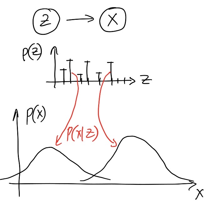
Apart from the learning problem, which involves estimating the whole joint distribution, there exists another problem that is worth solving on its own - the inference problem, i.e., estimating the latent factor given an observation. For examples, we may want to estimate “pose” of an object given its image in an unsupervised way, OR, estimating identity of a person given his/her facial photograph (our last example). Although we have seen how to perform inference in the EM algorithm, I am rewriting it here for convenience.

Taking up the same example of latent variable (i.e., $Z\to X$), we infer $Z$ as

$$\mathbb{P}(Z|X)=\frac{\mathbb{P}(X,Z)}{\mathbb{P}(X)}=\frac{\mathbb{P}(X,Z)}{\sum _Z\mathbb{P}(X,Z)}$$

This quantity is also called the posterior.

For continuos $Z$, we have integral instead of summation

$$\mathbb{P}(Z|X)=\frac{\mathbb{P}(X,Z)}{\mathbb{P}(X)}=\frac{\mathbb{P}(X,Z)}{{\int }_Z\mathbb{P}(X,Z)}$$

If you are a keen observer, you might notice an appearent problem with the inference - the inference will be computationally intractable as it involves a summation/integration over a high dimensional vector with potentially unbounded support. For example, if the latent variable denotes a continuous “pose” vector of length $d$, the denominator will contain a $d$-dimensional integral over $(-\mathrm{\infty },\mathrm{\infty }{)}^d$. At this point, as you might understand that even EM algorithm suffers from intractability problem.

Variational Inference (VI) comes to rescue

Finally, here we are. This is the one alogrithm I was most excited to explain because this is what some of the ground-breaking ideas of this field born out of. Variational Inference (VI), although there in the literature for a long time, has recently shown very promising results on problems involving latent variables and deep structure. In the next post, I will go into some of those specific algorithms, but not today. In this article, I will go over the basic framework of VI and how it works.

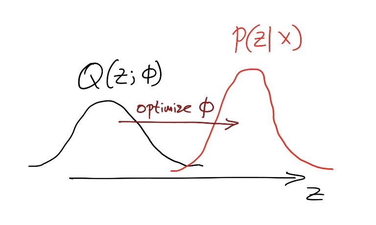
The idea is really simple: If we can’t get a tractable closed-form solution for $\mathbb{P}(Z|X)$, we’ll approximate it.

Let the approximation be $\mathbb{Q}(Z;\varphi )$ and we can now form this as an optimization problem:

$${\mathbb{Q}}^{\ast }(Z)=arg\underset{\varphi }{min}\mathbb{K}\mathbb{L}[\mathbb{Q}(Z;\varphi )||\mathbb{P}(Z|X)]$$

By choosing a family of distribution $\mathbb{Q}(Z;\varphi )$ flexible enough to model $\mathbb{P}(Z|X)$ and optimizing over $\varphi$, we can push the approximation towards the real posterior. $\mathbb{K}\mathbb{L}(\cdot \parallel \cdot )$ is KL-divergance, a distance between two probability distributions.

Fig.4: Variational approximation of the true posterior

Now let’s expand the KL-divergence term

$$\mathbb{K}\mathbb{L}[\mathbb{Q}(Z;\varphi )||\mathbb{P}(Z|X)]$$

$$={\mathbb{E}}_{\mathbb{Q}}[\log \mathbb{Q}(Z;\varphi )]-{\mathbb{E}}_{\mathbb{Q}}[\log \mathbb{P}(Z|X)]$$

$$={\mathbb{E}}_{\mathbb{Q}}[\log \mathbb{Q}(Z;\varphi )]-{\mathbb{E}}_{\mathbb{Q}}[\log \frac{\mathbb{P}(X,Z)}{\mathbb{P}(X)}]$$

$$={\mathbb{E}}_{\mathbb{Q}}[\log \mathbb{Q}(Z;\varphi )]-{\mathbb{E}}_{\mathbb{Q}}[\log \mathbb{P}(X,Z)]+\log \mathbb{P}(X)$$

Although we can compute the first two terms in the above expansion, but oh lord ! the third term is the same annoying (intractable) integral we were avoiding before. What do we do now ? This seems to be a deadlock !

The Evidence Lower BOund (ELBO)

Please recall that our original objective was a minimization problem over $\mathbb{Q}(\cdot ;\varphi )$. We can pull a little trick here - we can optimize only the first two terms and ignore the third term. How ?

Because the third term is independent of $\mathbb{Q}(\cdot ;\varphi )$. So, we just need to minimize

$${\mathbb{E}}_{\mathbb{Q}}[\log \mathbb{Q}(Z;\varphi )]-{\mathbb{E}}_{\mathbb{Q}}[\log \mathbb{P}(X,Z)]$$

Or equivalently, maximize (just flip the two terms)

$$ELBO(\mathbb{Q})\triangleq {\mathbb{E}}_{\mathbb{Q}}[\log \mathbb{P}(X,Z)]-{\mathbb{E}}_{\mathbb{Q}}[\log \mathbb{Q}(Z;\varphi )]$$

This term, usually defined as ELBO, is quite famous in VI literature and you have just witnessed how it looks like and where it came from. Taking a deeper look into the $ELBO(\cdot )$ yields even further insight

$$ELBO(\mathbb{Q})={\mathbb{E}}_{\mathbb{Q}}[\log \mathbb{P}(X|Z)]+{\mathbb{E}}_{\mathbb{Q}}[\log \mathbb{P}(Z)]-{\mathbb{E}}_{\mathbb{Q}}[\log \mathbb{Q}(Z;\varphi )]$$

$$={\mathbb{E}}_{\mathbb{Q}}[\log \mathbb{P}(X|Z)]-\mathbb{K}\mathbb{L}[\mathbb{Q}(Z;\varphi )||\mathbb{P}(Z)]$$

Now, please consider looking at the last equation for a while because that is what all our efforts led us to. The last equation is totally tractable and also solves our problem. What it basically says is that maximizing $ELBO(\cdot )$ (which is a proxy objective for our original optimization problem) is equivalent to maximizing the conditional data likelihood (which we can choose in our graphical model design) and simultaneously pushing our approximate posterior (i.e., $\mathbb{Q}(;\varphi )$) towards a prior over $Z$. The prior $\mathbb{P}(Z)$ is basically how the true latent space is organized. Now the immediate question might arise: “Where do we get $\mathbb{P}(Z)$ from?”. The answer is, we can just choose any distribution as a hypothesis. It will be our belief of how the $Z$ space is organized.

Fig.5: Interpretation of ELBO

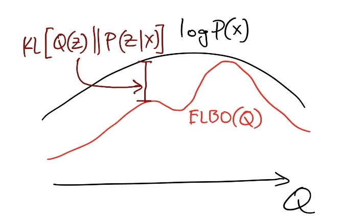
There is one more interpretation (see figure 5) of the KL-divergence expansion that is interesting to us. Rewriting the KL-expansion and substituting $ELBO(\cdot )$ definition, we get

$$\log \mathbb{P}(X)=ELBO(\mathbb{Q})+\mathbb{K}\mathbb{L}[\mathbb{Q}(Z;\varphi )||\mathbb{P}(Z|X)]$$

As we know that $\mathbb{K}\mathbb{L}(\cdot ||\cdot )\ge 0$ for any two distributions, the following inequality holds

$$\log \mathbb{P}(X)\ge ELBO(\mathbb{Q})$$

So, the $ELBO(\cdot )$ that we vowed to maximize is a lower bound on the observed data log likelihood. Thats amazing, isn’t it ! Just by maximing the $ELBO(\cdot )$, we can implicitely get closer to our dream of estimating maximum (log)-likelihood - tighter the bound, better the approximation.

---

Okay ! Way too much math for today. This is overall how the Variational Inference looks like. There are numerous directions of research emerged from this point onwards. Its impossible to talk about all of them. But few directions, which succeded to grab attention of the community with its amazing formulations and results will be discussed in later parts of the tutorial series. One of them being “Variational AutoEncoder” (VAE). Stay tuned.

References

1. “Variational Inference: A Review for Statisticians”, David M. Blei, Alp Kucukelbir, Jon D. McAuliffe
2. “Pattern Recognition and Machine Learning”, C.M. Bishop
3. “Machine Learning: A Probabilistic Perspective”, Kevin P. Murphy