Advanced Python: Bytecodes and the Python Virutal Machine (VM) - Part I

Over the years, Python has become one of the major general purpose programming language that the industry and academia care about. But even with a vast community around the language, very few of them are aware of how Python is actually executed on a computer system. Some of them have a vague idea of how Python is executed, which is partly because it’s totally possible to know nothing about it and still be a successful Python programmer. They believe that unlike C/C++, Python is “interpreted” instead of “compiled”, i.e. they are executed one statement at a time rather that converting down to some kind of machine code. It is not entirely correct. This post is targeted towards programmers with a fair knowledge of Python’s language fundamentals, to clear the fog around what really goes on when you hit python script.py. WARNING: This is a fairly advanced topic and not for beginners.

What exactly we mean by the term Python :

Before we begin, I want to clear out a very common misconception. It is widely assumed among beginner Python programmers that the term Python refers to the language and/or it’s interpreter - that’s NOT technically correct. The term Python should refer to the “language” only, i.e., the grammar of the language and NOT the interpreter (the command line tool named python or python2.7 or python3.5 etc) that runs your python code. The interpreter you have access to is one of the implementations of the language grammar. There are more than one implementations of Python language interpreter:

1. CPython: A python interpreter written in C language
2. PyPy: A python interpreter with Just-in-time (JIT) compilation
3. Jython: A python interpreter that uses the Java Virtual Machine (JVM)
4. IronPython: A python interpreter that uses .NET framework

Now, it so happened that CPython is the implementation provided by the same group of people (including creator Guido Van Rossum) who are responsible for defining Python’s language grammar as a reference implementation. For several reasons, CPython is also the mostly used Python interpreter out there. So that’s why it’s fairly reasonable, although not technically correct, to refer to the “Python language” plus the CPython interpreter collectively as Python. I am going to follow this convention throughout these tutorials.

Apart from clearing the misconception, there is another reason I said all this at the very beginning. The materials I am going to present in this tutorial are highly dependent of which interpreter we are talking about. Almost everything I am gonna talk about here is specific to CPython interpreter.

Compilers vs Interpreters :

Before we describe Python’s execution process, it is required to have a clear idea about what Compilers and Interpreters are and how they differ. In simple terms:

1. Compilers are programs that consume a program written in high level language and converts them down to machine code which the native CPU is capable of running directly. C/C++ is a typical example of a “compiled” language which can be compiled by one of severals implementations of a C/C++ compiler (famous ones being gcc by GNU, msvc by Microsoft, Clang by Google, icc by Intel etc).

2. Interpreters, on the other hand, reads a high level source program statement-by-statement and executes them in an interpreter while keeping some kind of context alive. But very often, a so-called “interpreted language” is not truly interpreted from their source program, rather they are interpreted after the source has been converted down to some form of intermediate representation. Precisely, Python falls into this category.

Bytecodes: The Intermediate Representation

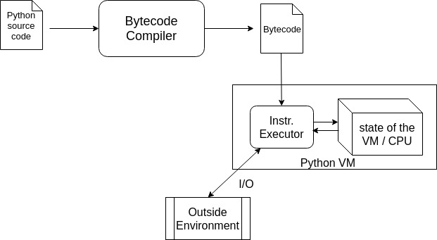
Python follows a two step process: first one being a Compilation step that converts our nice and sweet looking Python source code into an intermediate form called Python bytecode. Let’s see how they look like. This little function

def f(x):
    # computes (x^12 + x)
    y = x ** 12
    return x + y

is compiled by CPython’s Bytecode compiler and produces

124, 0,
100, 1,
19, 0,
125, 1,
124, 0,
124, 1,
23, 0,
83, 0

Wow, they are so readable, isn’t it ? Huhh, kidding. Of course you cannot make sense of them like this. Let’s make it a bit more readable:

LOAD_FAST         0
LOAD_CONST        1
BINARY_POWER
STORE_FAST        1
LOAD_FAST         0
LOAD_FAST         1
BINARY_ADD
RETURN_VALUE

If you’ve ever worked with assembly language before, you are likely to find similarities between assembly language and the above bytecode (the readable one). And and sequence of integers (124, 0, 100, ...) may also look like machine code to you. Guess what, you are kinda right. They are equivalent to assembly and machine code respectively. If you are wondering how CPython came up with this Bytecode representation, you should go through any good resource on general Compiler Theory because the way CPython generates Bytecodes is no different (but relatively simpler) than how a C/C++ compiler generates assembly code.

Design of the Bytecode instruction set:

Looking at “LOAD_FAST”, “LOAD_CONST”, “BINARY_POWER”, “BINARY_ADD” and all those instructions, you might have already suspected that there must be a whole bunch of these. The entire list of CPython’s bytecodes are available in Python’s official documentation. The exact design of CPython’s bytecodes instruction set is again version dependent - they might change slightly from version to version. So, for the sake of simplicity, I am choosing CPython 3.6 for this demonstration.

In CPython 3.6, all bytecode instructions are of exactly two bytes long and have a format of

<INSTRUCTION> <ARGUMENT>

with one byte each. There is a total of 118 unique instructions in the set, among which, some of the instructions do not care about it’s argument as in they don’t have an argument. The second byte of such instructions are to be ignored by the VM. Every (human readable) instruction has integer representation (of course below 256, because it’s one byte). One can easily figure out the mapping for few of them by comparing the above not-so-readable and the readable version of the bytecode.

LOAD_FAST -> 124
LOAD_CONST -> 100
BINARY_POWER -> 19
...

There is a magic number defined along with the instruction set which determines whether a particular instruction requires argument or not. If the integer representation of an instruction is less than that number, it doesn’t have an argument - that’s the rule. In CPython 3.6, the magic number happens to be 90. The “BINARY_POWER” does not have an argument (or rather ignores it) because it’s byte representation (i.e., 19) is less than 90.

Now that you have seen it all, let me disclose how I compiled the python program and where did I get these bytecodes from. It turns out that it’s very easy. The python interpreter allows you to peek into the bytecode from higher level python source code itself.

>>> def f(x):
        y = x ** 12
        return x + y

>>> f.__code__
<code object f at 0x7f976d44e810, file "<...>", line 1>

See that f.__code__ attribute - that’s the gateway to the compiled bytecode. f.__code__ contains some metadata as well. The raw bytecode can be retrieved from

>>> f.__code__.co_code
b'|\x00d\x01\x13\x00}\x01|\x00|\x01\x17\x00S\x00'

As it happened, some of the bytes are non-printable characters so they won’t show up properly on the screen. Converting them to integers will produce

>>> [int(x) for x  in f.__code__.co_code]
[124, 0, 100, 1, 19, 0, 125, 1, 124, 0, 124, 1, 23, 0, 83, 0]

the exact sequence of bytes I showed earlier.

Where are the data used by the program ?

If you are a keen observer and had been looking at the bytecode since you saw it, you might have noticed that there is a discrepancy between the generated bytecode and the python source program. The “data” used by the program are missing. In this example, I have used a numeric value (12) in the statement y = x ** 12. Did you see that anywhere in the compiled bytecode ? The point here is, the code and the data of a source program lives in different objects. Just like __code__.co_code holds the raw bytecode instructions, there are few other attributes that are responsible for holding the data. One of them is

>>> f.__code__.co_consts
(None, 12)

which holds our numeric value (12) and a (useless) None. I will explain the other ones in another tutorial as they are not really used in our running example. This way of looking at bytecodes is fine, but for more in-depth understanding you need something more convenient - the standard library module called dis will help you:

>>> import dis # basically 'disassembler'
>>> dis.dis(f)
  2           0 LOAD_FAST                0 (x)
              2 LOAD_CONST               1 (12)
              4 BINARY_POWER
              6 STORE_FAST               1 (y)

  3           8 LOAD_FAST                0 (x)
             10 LOAD_FAST                1 (y)
             12 BINARY_ADD
             14 RETURN_VALUE

If you are really interested, go explore the dis module. From my side, a detailed explanation of this output is the agenda of the next tutorial in this series.

After seeing all these, an immediate question you might be tempted to ask is whether these machine code lookalikes can be executed directly on a physical system ? Unfortunately, NO, they cannot. These bytecodes are not designed to be ran on any physical CPU. Rather, they are specially crafted to be consumed by a piece of software which is the second part of Python’s execution process - the Virtual Machine (VM).

Python VM: Interpreting the Bytecodes

The Python Virtual Machine (VM) is a separate program which comes into picture after the Bytecode compiler has generated the bytecode. It is literally a simulation of a physical CPU - it has software defined stacks, instruction pointer (IP) and what not. Although, other virtual machines may have a lot of other components like registers etc., but the CPython VM is entirely based on a stack data structure which is why it is often referred to as a “stack-based” virtual machine.

If you cannot get a feel of what it is, I have a dumb little code to show how Python VM is literally implemented. In reality, CPython VM is implemented in C but for simplicity, I am showing an equivalent but terribly simplified version in python itself:

def action_BINARY_POWER(args, state):
    # ...
def action_RETURN_VALUE(args, state):
    # ...
INSTRUCTION_SET = {
    'BINARY_POWER': action_BINARY_POWER,
    'RETURN_VALUE': action_RETURN_VALUE,
    # ... a lot of these
    # ...
    'LOAD_CONST': # ...
}
class VirtualCPU:

    # Power-ON for the CPU
    def __init__(self):
        # these represents the 'state' of the virtual CPU

        # a simulated stack
        self.stack = Stack()
        # a simulated instruction pointer
        self.IP = 0

    # executes one instruction
    def exec_instruction(self, instruction, instruction_arg):
        action = INSTRUCTION_SET[instruction]
        action(instruction_arg, (self.stack, self.IP))

    # a running CPU
    def main_loop(self, stream_of_instructions):
        for instruction, argument in stream_of_instructions:
            self.exec_instruction(instruction, argument)

# an instance
cpu = VirtualCPU()

Please spend a minute to digest this. This is almost how the Python VM is implemented internally. Upon feeding a stream of (instruction, argument) pair, the VirtualCPU.main_loop() will keep iterating over them and execute one instruction at a time. If the main_loop() is fed with our previously compiled Bytecode program in a properly arranged data structure

cpu.main_loop([
        ('LOAD_FAST', 0),
        ('LOAD_CONST', 1),
        ('BINARY_POWER', None),
        ('STORE_FAST', 1),
        ('LOAD_FAST', 0),
        ('LOAD_FAST', 1),
        ('BINARY_ADD', None),
        ('RETURN_VALUE', None)
    ])

cpu.exec_instruction(instruction, instruction_arg) will take one instruction and resolve the corresponding action routine (one of the action_* functions) from a well-defined set of instruction-action pairs and execute that. Notice, the action_*() functions take the state of the CPU as input (in this case the stack and the IP) because it has to manipulate the CPU’s state. This is exactly what happens inside a real CPU.

For a bit more clarity on the action_* functions, let’s have a look at one instruction and it’s corresponding action function in a little more detail. Consider the “BINARY_ADD” instruction: it pops off two elements from the stack and pushes their addition result on the stack. This is roughly how it is implemented:

def action_BINARY_ADD(args, state):
    # 'args' is None - that's useless here
    
    stack, ip = state
    addend = stack.pop()
    augend = stack.pop()

    stack.push(augend + addend) # manipulates the state

    ip += 1 # manipulates the state

Please remember, this is just to show you the logical steps - the actual CPython interpreter is way more complicated, and of course, written in C.

Cached Bytecodes: The .pyc files

In principle, every time you run a script, python has to go through both Compilation and Interpretation steps. If you are running the same script over and over again, it is wasteful to execute bytecode compilation every time because a particular python source code will produce the same bytecode every time you do the compilation.

CPython uses a caching mechanism to avoid this. It writes down the bytecode the first time you load a module - yes, it happens at module level. If you load it again without modification, it will read the cached bytecode and go through the interpretation process only. These cached bytecodes are kept inside .pyc files which you must have seen before:

prompt $ tree
.
├── __pycache__
│   └── module.cpython-36.pyc # THIS one
└── module.py

1 directory, 2 files

The bytecodes along with the data are serialized into these .pyc files using a very special serialization format called marshal which is strictly an internal format to python interpreter implementation and not supposed to be used by application programs. If you really want to know more about marshal, see Stephane Wirtel’s video on Youtube.