Introduction to Probabilistic Programming

Welcome to another tutorial about probabilistic models, after a primer on PGMs and VAE. However, I am particularly excited to discuss a topic that doesn’t get as much attention as traditional Deep Learning does. The idea of Probabilistic Programming has long been there in the ML literature and got enriched over time. Before it creates confusion, let’s declutter it right now - it’s not really writing traditional “programs”, rather it’s building Probabilistic Graphical Models (PGMs), but equipped with imperative programming style (i.e., iterations, branching, recursion etc). Just like Automatic Differentiation allowed us to compute derivative of arbitrary computation graphs (in PyTorch, TensorFlow), Black-box methods have been developed to “solve” probabilistic programs. In this post, I will provide a generic view on why such a language is indeed possible and how such black-box solvers are materialized. At the end, I will also introduce you to one such Universal Probabilistic Programming Language, Pyro, that came out of Uber’s AI lab and started gaining popularity.

Overview

Before I dive into details, let’s get the bigger picture clear. It is highly advisable to read any good reference about PGMs before you proceed - my previous article for example.

Generative view & Execution trace

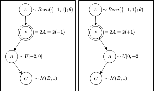
Probabilistic Programming is NOT really what we usually think of as programming - i.e., completely deterministic execution of hard-coded instructions which does exactly what its told and nothing more. Rather it is about building PGMs (must read this) which models our belief about the data generation process. We, as users of such language, would express a model in an imperative form which would encode all our uncertainties in the way we want. Here is a (Toy) example:

def model(theta):
    A = Bernoulli([-1, 1]; theta)
    P = 2 * A
    if A == -1:
        B = Uniform(P, 0)
    else:
        B = Uniform(0, P)
    C = Normal(B, 1)
    return A, P, B, C

If you assume this to be valid program (for now), this is what we are talking about here - all our traditional “variables” become “random variables” (RVs) and have uncertainty associated with them in the form of probability distributions. Just to give you a taste of its flexibility, here’s the constituent elements we encountered

1. Various different distributions are available (e.g., Normal, Bernoulli, Uniform etc.)
2. We can do deterministic computation (i.e., \(P = 2 * A\))
3. Condition RVs on another RVs (i.e., \(C\vert B \sim \mathcal{N}(B, 1)\))
4. Imperative style branching allows dynamic structure of the model …

Below is a graphical representation of the model defined by the above program.

Just like the invocation of a traditional compiler on a traditional program produces the desired output, this (probabilistic) program can be executed by means of “ancestral sampling”. I ran the program 5 times and each time I got samples from all my RVs. Each such “forward” run is often called an execution trace of the model.

>>> for _ in range(5):
        print(model(0.5))
(1.000, 2.000, 0.318, -0.069)
(-1.000, -2.000, -1.156, -2.822)
(1.000, 2.000, 0.594, 0.865)
(1.000, 2.000, 1.100, 1.079)
(-1.000, -2.000, -0.262, -0.403)

This is the so called “generative view” of a model. We typically use the leaf-nodes of PGMs as our observed data. And rest of the graph can be the “latent factors” of the model which we either know or want to estimate. In general, a practical PGM can often be encapsulated as a set of latent nodes \(\mathbf{Z} \triangleq \{ Z_1, Z_2, \cdots, Z_H \}\) and visible nodes \(\mathbf{X} \triangleq \{ X_1, X_2, \cdots, X_V \}\) related probabilistically as
\[ \mathbf{Z} \rightarrow \mathbf{X} \]

Training and Inference

From now on, we’ll use the general notation rather than the specific example. The model may be parametric. For example, we had the bernoulli success probability \(\theta\) in our toy example. The full joint probability is given as

\[ \mathbb{P}_{\theta}(\mathbf{Z}, \mathbf{X}) = \mathbb{P}_{\theta}(\mathbf{Z}) \cdot \mathbb{P}_{\theta}(\mathbf{X}\vert \mathbf{Z}) \]

We would like to do two things: 1. Estimate model parameters \(\theta\) from data 2. Compute the posterior, i.e., infer latent variables given data

As discussed in my PGM article, both of them are infeasible due to the fact that 1. Log-likehood maximization is not possible because of the presence of latent variables 2. For continuous distributions on latent variables, the posterior is intractible

The way forward is to take help of Variational Inference and maximize our very familiar Evidence Lower BOund (ELBO) loss to estimate the model parameters and also a set of variational parameters which help building a proxy for the original posterior \(\mathbb{P}_{\theta}(\mathbf{Z}\vert \mathbf{X})\). Mathematically, we choose a known and tractable family of distribution \(\mathbb{Q}_{\phi}(\mathbf{Z})\) (parameterized by variational parameters \(\phi\)) to approximate the posterior. The learning process is facilitated by maximizing the following

\[ \mathrm{ELBO}(\theta, \phi) \triangleq \mathbb{E}_{\mathbb{Q}_{\phi}} \bigl[\log \mathbb{P}_{\theta}(\mathbf{Z}, \mathbf{X}) - \log \mathbb{Q}_{\phi}(\mathbf{Z}) \bigr] \]

by estimating gradients w.r.t all its parameters

\[\tag{1} \nabla_{[\theta, \phi]} \mathrm{ELBO}(\theta, \phi) \]

Black-Box Variational Inference

If you have gone through my PGM article, you might think you’ve seen these before. Actually, you’re right ! There is really nothing new to this. What we really need for establishing a Probabilistic Programming framework is a unified way to implement the ELBO optimization for ANY given problem. And by “problem” I mean the following:

1. A model specification \(\mathbb{P}_{\theta}(\mathbf{Z}, \mathbf{X})\) written in a probabilistic language (like we saw before)
2. An optional (parameterized) “Variational Model” \(\mathbb{Q}_{\phi}(\mathbf{Z})\), famously known as a “Guide”
3. And .. the observed data \(\mathcal{D}\), of course

But, how do we compute (1) ? The appearent problem is that gradient w.r.t. \(\phi\) is required but it appears in the expectation itself. To mitigate this, we make use of the famous trick known as the “log-derivative” trick (it actually has many other names like REINFORCE etc). For notational simplicy let’s denote \(f(\mathbf{Z}, \mathbf{X}; \theta, \phi) \triangleq \log \mathbb{P}_{\theta}(\mathbf{Z}, \mathbf{X}) - \log \mathbb{Q}_{\phi}(\mathbf{Z})\) and continue from (1)

\[ \sum_{\mathbf{Z}} \nabla_{[\theta, \phi]} \bigg[ \mathbb{Q}_{\phi}(\mathbf{Z}) \cdot f(\mathbf{Z}, \mathbf{X}; \theta, \phi) \bigg] \] \[ =\sum_{\mathbf{Z}} \bigg[ \nabla_{\phi} \mathbb{Q}_{\phi}(\mathbf{Z}) \cdot f(\mathbf{Z}, \mathbf{X}; \theta, \phi) +\mathbb{Q}_{\phi}(\mathbf{Z}) \cdot \nabla_{[\theta, \phi]}f(\mathbf{Z}, \mathbf{X}; \theta, \phi) \bigg] \]

\[ =\sum_{\mathbf{Z}} \bigg[ {\color{red}\mathbb{Q}_{\phi}(\mathbf{Z})} \cdot \frac{\nabla_{\phi} \mathbb{Q}_{\phi}(\mathbf{Z})}{{\color{red}\mathbb{Q}_{\phi}(\mathbf{Z})}} \cdot f(\mathbf{Z}, \mathbf{X}; \theta, \phi) +\mathbb{Q}_{\phi}(\mathbf{Z}) \cdot \nabla_{[\theta, \phi]}f(\mathbf{Z}, \mathbf{X}; \theta, \phi) \bigg] \]

\[ =\sum_{\mathbf{Z}} \mathbb{Q}_{\phi}(\mathbf{Z}) \cdot \bigg[ {\color{red}\nabla_{\phi} \log\mathbb{Q}_{\phi}(\mathbf{Z})} \cdot f(\mathbf{Z}, \mathbf{X}; \theta, \phi) +\nabla_{[\theta, \phi]}f(\mathbf{Z}, \mathbf{X}; \theta, \phi) \bigg] \]

\[\tag{2} = \mathbb{E}_{\mathbb{Q}_{\phi}} \bigg[ \nabla_{[\theta, \phi]} \bigg( \underbrace{\log\mathbb{Q}_{\phi}(\mathbf{Z}) \cdot \overline{f(\mathbf{Z}, \mathbf{X}; \theta, \phi)} +f(\mathbf{Z}, \mathbf{X}; \theta, \phi)}_\text{Surrogate Objective} \bigg) \bigg] \]

Eq. (2) shows that the trick helped the \(\nabla_{[\theta, \phi]}\) to penetrate the \(\mathbb{E}[\cdot]\), but in the process, it changed the original \(f\) with a “surrogate function” \(f_{surr} \triangleq \overline{f}\cdot\log\mathbb{Q}+f\) where the bar protects a quantity from differentiation. Equation (2) is all we need - it provides an insight on how to make the gradient estimation practical. In fact, it can be proven theoretically that this gradient is an unbiased estimate of the true gradient in Equation (1).

Succinctly, we run the Guide \(L\) times to record a set of \(L\) execution-traces (i.e., samples \(\mathbf{\widehat{Z}}\sim\mathbb{Q}_{\phi}\)) and compute the following Monte-Carlo approximation to Equation (2)

\[\tag{3} \nabla_{[\theta, \phi]} \mathrm{ELBO}(\theta, \phi) \approx \frac{1}{L} \sum_{\mathbf{\widehat{Z}}\sim\mathbb{Q}_{\phi}} \left[ \nabla_{[\theta, \phi]} f_{surr}(\mathbf{\widehat{Z}}, \mathcal{D}) \right]_{\theta=\theta_{old}, \phi=\phi_{old}} \]

The nice thing about Equation (2) (or equivalently Equation (3)) is we got the differentiation operator right on top of a deterministic function (i.e., \(f_{surr}\)). It means we can construct \(f_{surr}\) as a computation graph and take advantage of modern day automatic differentaition engines. Figure 1 shows how the computation graph and the graphical model are linked

Figure 1: Graphical model & the computational graph

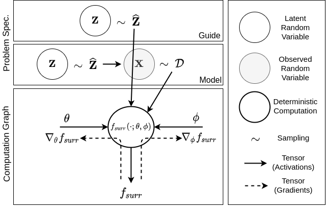
Last but not the least, let’s look at the function \(f_{surr}\) which is basically built on the log-density terms \(\log \mathbb{P}_{\theta}(\mathbf{Z}, \mathbf{X})\) and \(\log \mathbb{Q}_{\phi}(\mathbf{Z})\). We need a way to compute them flexibly. Please remember that the model and guide is written in a language and hence we have access to their graph-structure. A clever software implementation can harness this structure to estimate the log-densities (and eventually \(f_{surr}\)).

I claimed before that the gradient estimates are unbiased. However, such generic way of computing the gradient introduces high variance in the estimate and make things unstable for complex models. There are few tricks used widely to get around them. But please note that such tricks always exploits model-specific structure. Three such tricks are presented below.

I. Re-parameterization

We might get lucky that \(\mathbb{Q}_{\phi}(\mathbf{Z})\) is re-parameterizable. What that means is the expectation w.r.t \(\mathbb{Q}_{\phi}(\mathbf{Z})\) can be made free of its parameters and by doing so the gradient operator can be pushed inside without going through the log-derivative trick. So, let’s step back a bit and consider the original ELBO gradient in (1). Assuming re-parameterizable nature, the following can be done \[ \nabla_{[\theta, \phi]} \mathbb{E}_{\mathbb{Q}_{\phi}} \bigg[\log \mathbb{P}_{\theta}(\mathbf{Z}, \mathbf{X}) - \log \mathbb{Q}_{\phi}(\mathbf{Z}) \bigg] = \nabla_{[\theta, \phi]} \mathbb{E}_{Q(\mathbf{\epsilon})} \bigg[\log \mathbb{P}_{\theta}(G_{\phi}(\epsilon), \mathbf{X}) - \log \mathbb{Q}_{\phi}(G_{\phi}(\epsilon)) \bigg] \] \[ = \mathbb{E}_{Q(\mathbf{\epsilon})} \bigg[\nabla_{[\theta, \phi]} \bigg( \log \mathbb{P}_{\theta}(G_{\phi}(\mathbf{\epsilon}), \mathbf{X}) - \log \mathbb{Q}_{\phi}(G_{\phi}(\epsilon)) \bigg) \bigg] \]

Where \(Q(\mathbf{\epsilon})\) is an independent source of randomness. Computing this expectation with empirical average (just like Eq.2) gives us a better (variance reduced) estimate of the true gradient of ELBO.

II. Rao-Blackwellization

This is another well-known variance reduction technique. It is a bit mathematically rigorous, so I will explain it simply without making it confusing. This requires the full variational distributions to have some kind of factorization. A specific case is when we have mean-field assumption, i.e.

\[ \mathbb{Q}_{\phi}(\mathbf{Z}) = \prod_i Q_{\phi_i}(Z_i) \]

With a little effort, we can pull out the gradient estimator for each of these \(\phi_i\) parameters from (2). They look something like this

\[ \nabla_{\phi_i} \mathrm{ELBO}(\theta, \phi) = \mathbb{E}_{\mathbb{Q}_{\phi}} \bigg[ \nabla_{\phi_i} \log\mathbb{Q}_{\phi_i}(Z_i) \cdot \bigg( \overline{\log \mathbb{P}_{\theta}(\mathbf{Z}, \mathbf{X}) - \log \mathbb{Q}_{\phi}(\mathbf{Z})} \bigg) +\cdots \bigg] \]

The reason why the quantity under bar still has all the factors because it is immune to gradient operator. Also because the expectation is outside the gradient operator, it contains all factors. At this point, the Rao-Blackwellization offers a variance-reduced estimate of the above gradient, i.e.,

\[ \nabla_{\phi_i} \mathrm{ELBO}(\theta, \phi) \approx \mathbb{E}_{\mathbb{Q}_{\phi}^{(i)}} \bigg[ \nabla_{\phi_i} \log\mathbb{Q}_{\phi_i}(Z_i) \cdot \bigg( \overline{\log \mathbb{P}^{(i)}_{\theta}(\mathbf{Z}^{(i)}, \mathbf{X}) - \log \mathbb{Q}_{\phi_i}(Z_i)} \bigg) +\cdots \bigg] \]

where \(\mathbf{Z}^{(i)}\) is the set of variables that forms the “markov blanket” of \(Z_i\) w.r.t to the structure of guide, \(\mathbb{Q}_{\phi}^{(i)}\) is the part of the variational distribution that depends on \(\mathbf{Z}^{(i)}\) and \(\mathbb{P}^{(i)}_{\theta}(\mathbf{Z}^{(i)}, \cdot)\) is the factors of the model that involves \(\mathbf{Z}^{(i)}\).

III. Explicit enumeration for Discrete RVs

While exploiting the graph structure of the guide while simplifying (1), we might end up getting a term like this due to factorization in the guide density

\[ \mathbb{E}_{Z_i\sim\mathbb{Q}_{\phi_i}(Z_i)} \bigl[ f(\cdot) \bigr] \]

If it happens that the variable \(Z_i\) is discrete with the size of its state space reasonably small (e.g., a \(d=5\) dimensional binary RV has \(2^5 = 32\) states), we can replace sampling-based empirical expectations with true expectation where we have to evaluate a sum over its entire state-space

\[ \sum_{Z_i} \mathbb{Q}_{\phi_i}(Z_i)\cdot f(\cdot) \]

So make sure the state-space is resonable in size. This helps reducing the variance quite a bit.

Whew ! That’s a lot of maths. But good thing is, you hardly ever have to think about them in detail because software engineers have put tremendous effort to make these algorithms as easily accessible as possible via libraries. One of them we are going to have a brief look on.

Pyro: Universal Probabilistic Programming

Pyro is a probabilistic programming framework that allows users to write flexible models in terms of a simple API. Pyro is written in Python and uses the popular PyTorch library for its internal representation of computation graph and as auto differentiation engine. Pyro is quite expressive due to the fact that it allows the model/guide to have fully imperative flow. It’s core API consists of these functionalities

1. pyro.param() for defining learnable parameters.
2. pyro.dist contains a large collection of probability distribution.
3. pyro.sample() for sampling from a given distribution.

Let’s take a concrete example and work it out.

Problem: Mixture of Gaussian

MoG (Mixture of Gaussian) is a realatively simple but widely studied probabilistic model. It has an important application in soft-clustering. For the sake of simplicity we assume we only have two mixtures. The generative view of the model is basically this: we flip a coin (latent) with bias \(\rho\) and depending on the outcome \(C\in \{ 0, 1 \}\) we sample data from either of the two gaussian \(\mathcal{N}(\mu_0, \sigma_0)\) and \(\mathcal{N}(\mu_1, \sigma_1)\)

\[ C_i \sim Bernoulli(\rho) \\ X_i \sim \mathcal{N}(\mu_{C_i}, \sigma_{C_i}) \]

where \(i = 1 \cdots N\) is data index, \(\theta \triangleq \{ \rho, \mu_1, \sigma_1, \mu_2, \sigma_2 \}\) is the set of model parameters we need to learn. This is how you write that in Pyro:

def model(data): # Take the observation
    # Define coin bias as parameter. That's what 'pyro.param' does
    rho = pyro.param("rho", # Give it a name for Pyro to track properly
        torch.tensor([0.5]), # Initial value
        constraint=dist.constraints.unit_interval) # Has to be in [0, 1]
    # Define both means and std with random initial values
    means = pyro.param("M", torch.tensor([1.5, 3.]))
    stds = pyro.param("S", torch.tensor([0.5, 0.5]),
        constraint=dist.constraints.positive) # std deviation cannot be negative

    with pyro.plate("data", len(data)): # Mark conditional independence
        # construct a Bernoulli and sample from it. 
        c = pyro.sample("c", dist.Bernoulli(rho)) # c \in {0, 1}
        c = c.type(torch.LongTensor)
        X = dist.Normal(means[c], stds[c]) # pick a mean as per 'c'
        pyro.sample("x", X, obs=data) # sample data (also mark it as observed)

Due to the discrete and low dimensional nature of the latent variable \(C\), this problem is in general tracktable in terms of computing posterior. But let’s assume it is not. The true posterior \(\mathbb{P}(C_i\vert X_i)\) is the quantity known as “assignment” that reveals the latent factor, i.e., what was the coin toss result when a given \(X_i\) was sampled. We define a guide on \(C\), parameterized by variational parameters \(\phi \triangleq \{ \lambda_i \}_{i=1}^N\)

\[ C_i \sim Bernoulli(\lambda_i) \]

In Pyro, we define a guide that encodes this

def guide(data): # Guide doesn't require data; just need the value of N
    with pyro.plate("data", len(data)): # conditional independence
        # Define variational parameters \lambda_i (one for every data point)
        lam = pyro.param("lam",
            torch.rand(len(data)), # randomly initiallized
            constraint=dist.constraints.unit_interval) # \in [0, 1]
        c = pyro.sample("c", # Careful, this name HAS TO BE same to match the model
            dist.Bernoulli(lam))

We generate some synthetic data from the following simualator to train our model on.

def getdata(N, mean1=2.0, mean2=-1.0, std1=0.5, std2=0.5):
    D1 = np.random.randn(N//2,) * std1 + mean1
    D2 = np.random.randn(N//2,) * std2 + mean2
    D = np.concatenate([D1, D2], 0)
    np.random.shuffle(D)
    return torch.from_numpy(D.astype(np.float32))

Finally, Pyro requires a bit of boilerplate to setup the optimization

data = getdata(200) # 200 data points
pyro.clear_param_store()
optim = pyro.optim.Adam({})
svi = pyro.infer.SVI(model, guide, optim, infer.Trace_ELBO())

for t in range(10000):
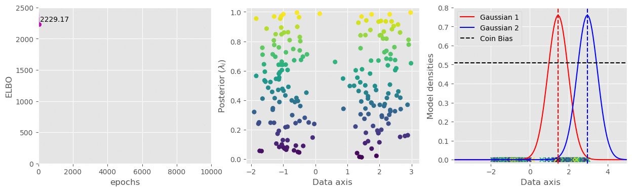
    svi.step(data)

That’s pretty much all we need. I have plotted the (1) ELBO loss, (2) Variational parameter \(\lambda_i\) for every data points, (3) The two gaussians in the model and (4) The coin bias as the training progresses.

The full code is available in this gist: https://gist.github.com/dasayan05/aca3352cd00058511e8372912ff685d8.

---

That’s all for today. Hopefully I was able to convey the bigger picture of probabilistic programming which is quite useful for modelling lots of problems. The following references the sources of information while writing the article. Interested readers are encouraged to check them out.

1. Pyro’s VI tutorial
2. Black Box variational inference
3. Gradient Estimation Using Stochastic Computation Graphs
4. Deep Probabilistic Programming
5. Pyro: Deep Universal Probabilistic Programming

Figure 1: Graphical model & the computational graph