Generative modelling is one of the seminal tasks for understanding the distribution of natural data. VAE, GAN and Flow family of models have dominated the field for last few years due to their practical performance. Despite commercial success, their theoretical and design shortcomings (intractable likelihood computation, restrictive architecture, unstable training dynamics etc.) have led to the developement of a new class of generative models named “Diffusion Probabilistic Models” or DPMs. Diffusion Models, first proposed by Sohl-Dickstein et al. (2015), inspire from thermodynam diffusion process and learn a noise-to-data mapping in discrete steps, very similar to Flow models. Lately, DPMs have been shown to have some intriguing connections to Score Based Models (SBMs) and Stochastic Differential Equations (SDE). These connections have further been leveraged to create their continuous-time analogous. In this article, I will describe both the general framework of DPMs, their recent advancements and explore the connections to other frameworks. For the sake of readers, I will avoid gory details, rigorous mathematical derivations and use subtle simplifications in order to maintain focus on the core idea.
In case you haven’t checked the first part of this two-part blog, please read Score Based Models (SBMs).
What exactly do we mean by “Diffusion” ?
In thermodynamics, “Diffusion” refers to the flow of particles from high-density regions towards low-density regions. In the context of statistics, meaning of Diffusion is quite similar, i.e. the process of transforming a complex distribution \(p_{\mathrm{complex}}\) on \(\mathbb{R}^d\) to a simple (predefined) distribution \(p_{\mathrm{prior}}\) on the same domain. Succinctly, a transformation \(\mathcal{T}: \mathbb{R}^d \rightarrow \mathbb{R}^d\) such that
\[ \mathbf{x}_0 \sim p_{\mathrm{complex}} \implies \mathcal{T}(\mathbf{x}_0) \sim p_{\mathrm{prior}} \tag{1}\]
where the symbol \(\implies\) means “implies”. There is a formal way to come up with a specific specific \(\{ \mathcal{T}, p_{\mathrm{prior}} \}\) pair that satisfies Equation 1 for any distribution \(p_{\mathrm{complex}}\). In simple terms, we can take any distribution and transform it into a known (simple) density by means of a known transformation \(\mathcal{T}\). By “formal way”, I was referring to Markov Chain and its stationary distribution, which says that by repeated application of a transition kernel \(q(\mathbf{x} \vert \mathbf{x}')\) on the samples of any distribution would lead to samples from \(p_{\mathrm{prior}}(\mathbf{x})\) if the following holds
\[ p_{\mathrm{prior}}(\mathbf{x}) = \int q(\mathbf{x} \| \mathbf{x}') p_{\mathrm{prior}}(\mathbf{x}') d\mathbf{x}' \]
We can related our original diffusion process in Equation 1 with a markov chain by defining \(\mathcal{T}\) to be repeated application of the transition kernel \(q(\mathbf{x} \vert \mathbf{x}')\) over discrete time \(t\)
\[ \mathbf{x}_{t} \sim q(\mathbf{x} \vert \mathbf{x}' = \mathbf{x}_{t-1}),\ \forall t > 0 \tag{2}\]
From the properties of stationary distribution, we have \(\mathbf{x}_{\infty} \sim p_{\mathrm{prior}}\). In practice, we can keep the iterations to a sufficiently large finite number \(t = T\).
So far, we confirmed that there is indeed an iterative way (refer to Equation 2) to convert the samples from a complex distributions to a known (simple) prior. Even though we talked only in terms of generic densities, there is one very attractive choice of \(\{ q, p_{\mathrm{prior}} \}\) pair (showed in Sohl-Dickstein et al. (2015)) due to its simplicity and tractability
\[ q(\mathbf{x}_t \vert \mathbf{x}_{t-1}) = \mathcal{N}(\mathbf{x}_t; \sqrt{1 - \beta_t} \mathbf{x}_{t-1}, \beta_t \mathrm{I}) \\ q(\mathbf{x}_T) = p_{\mathrm{prior}}(\mathbf{x}_T) = \mathcal{N}(\mathbf{x}_T; \mathbf{0}, \mathrm{I}) \tag{3}\]
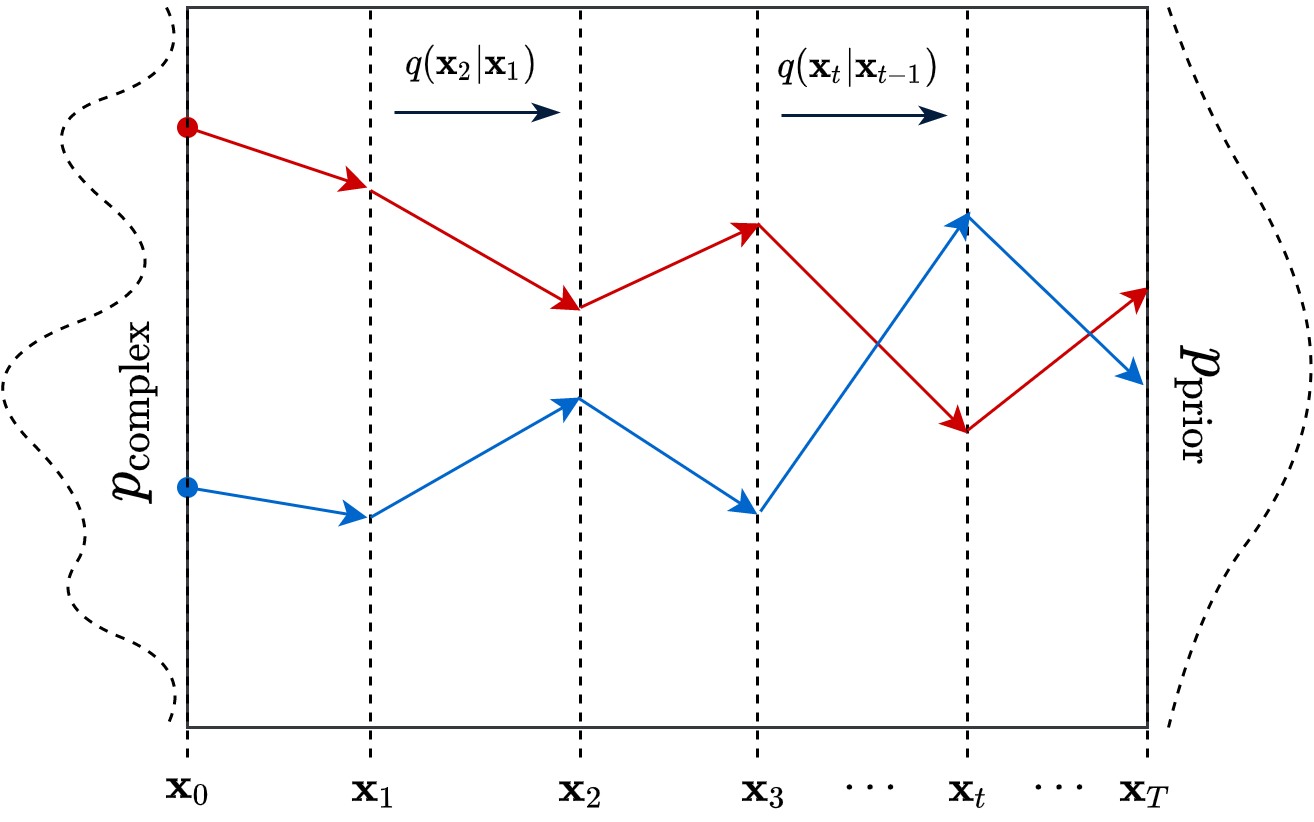
For obvious reason, its known as Gaussian Diffusion. I purposefuly changed the notations of the random variables to make it more explicit. \(\beta_t \in \mathbb{R}\) is a predefined decaying schedule proposed by Sohl-Dickstein et al. (2015). A pictorial depiction of the diffusion process is shown in Figure 1.
Generative modlling by undoing the diffusion
We proved the existence of a stochastic transform \(\mathcal{T}\) that gurantees the diffusion process in Eq 1. Please realize that the diffusion process does not depend on the initial density \(p_{\mathrm{complex}}\) (as \(t \rightarrow \infty\)) and the only requirement is to be able to sample from it. This is the core idea behind Diffusion Models - we use the any data distribution (let’s say \(p_{\mathrm{data}}\)) of our choice as the complex initial density. This leads to the forward diffusion process
\[ \mathbf{x}_0 \sim p_{\mathrm{data}} \implies \mathbf{x}_T = \mathcal{T}(\mathbf{x}_0) \sim \mathcal{N}(\mathbf{0}, \mathrm{I}) \]
This process is responsible for “destructuring” the data and turning it into an isotropic gaussian (almost structureless). Please refer to the figure below (red part) for a visual demonstration.
However, this isn’t very usefull by itself. What would be useful is doing the opposite, i.e. starting from isotropic gaussian noise and turning it into \(p_{\mathrm{data}}\) - that is generative modelling (blue part of the figure above). Since the forward process is fixed (non-parametric) and guranteed to exist, it is very much possible to invert it. Once inverted, we can use it as a generative model as follows
\[ \mathbf{x}_T \sim \mathcal{N}(\mathbf{0}, \mathrm{I}) \implies \mathcal{T}^{-1}(\mathbf{x}_T) \sim p_{\mathrm{data}} \]
Fortunately, the theroy of markov chain gurantees that for gaussian diffusion, there indeed exists a reverse diffusion process \(\mathcal{T}^{-1}\). The original paper from Sohl-Dickstein et al. (2015) shows how a parametric model of diffusion \(\mathcal{T}^{-1}_{\theta}\) can be learned from data itself.
Graphical model and training
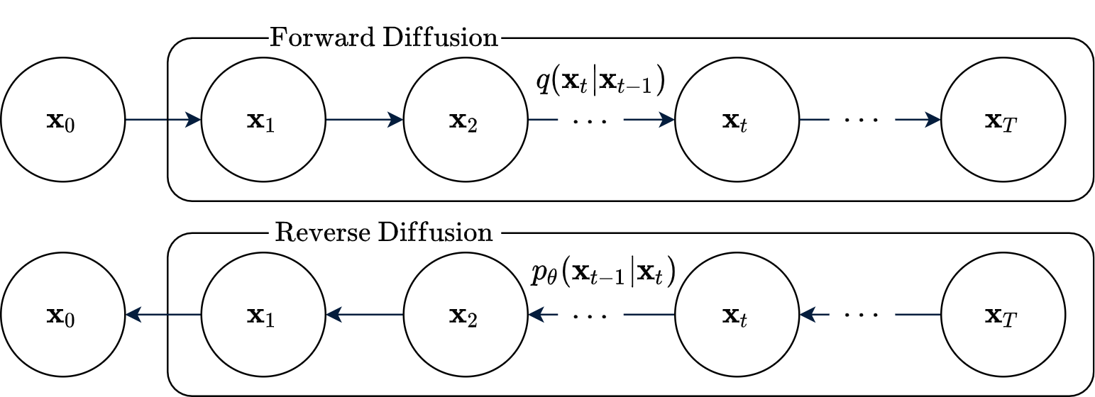
The stochastic “forward diffusion” and “reverse diffusion” processes described so far can be well expressed in terms of Probabilistic Graphical Models (PGMs). A series of \(T\) random variables define each of them; with the forward process being fully described by Equation 3. The reverse process is expressed by a parametric graphical model very similar to that of the forward process, but in reverse
\[ p(\mathbf{x}_T) = \mathcal{N}(\mathbf{x}_T; \mathbf{0}, \mathrm{I}) \\ p_{\theta}(\mathbf{x}_{t-1} \vert \mathbf{x}_t) = \mathcal{N}(\mathbf{x}_{t-1}; \mathbf{\mu}_{\theta}(\mathbf{x}_t, t), \mathbf{\Sigma}_{\theta}(\mathbf{x}_t, t)) \tag{4}\]
Each of the reverse conditionals \(p_{\theta}(\mathbf{x}_{t-1} \vert \mathbf{x}_t)\) are structurally gaussians and responsible for learning to revert each corresponding steps in the forward process, i.e. \(q(\mathbf{x}_t \vert \mathbf{x}_{t-1})\). The means and covariances of these reverse conditionals are neural networks with parameters \(\theta\) and shared over timesteps. Just like any other probabilistic models, we wish to minimize the negative log-likelihood of the model distribution under the expectation of data distribution
\[ \mathcal{L} = \mathbb{E}_{\mathbf{x}_0 \sim p_{\mathrm{data}}}\big[ - \log p_{\theta}(\mathbf{x}_0) \big] \]
which isn’t quite computable in practice due to its dependance on \((T-1)\) more random variables. With a fair bit of mathematical manipulations, Sohl-Dickstein et al. (2015) (section 2.3) showed \(\mathcal{L}\) to be a lower-bound of another easily computatable quantity
\[ \mathcal{L} \leq \mathbb{E}_{\mathbf{x}_0 \sim p_{\mathrm{data}},\ \mathbf{x}_{1:T} \sim q(\mathbf{x}_{1:T} | \mathbf{x}_0)} \bigg[ - \log p(\mathbf{x}_T) - \sum_{t\geq 1} \log \frac{p_{\theta}(\mathbf{x}_{t-1} \vert \mathbf{x}_t)}{q(\mathbf{x}_t \vert \mathbf{x}_{t-1})} \bigg] \]
which is easy to compute and optimize. The expectation is over the joint distribution of the entire forward process. Getting a sample \(\mathbf{x}_{1:T} \sim q(\cdot \vert \mathbf{x}_0)\) boils down to executing the forward diffusion on one sample \(\mathbf{x}_0 \sim p_{\mathrm{data}}\). All quantities inside the expectation are tractable and available to us in closed form.
Further simplification: Variance Reduction
Even though we can train the model with the lower-bound shown above, few more simplifications are possible. First one is due to Sohl-Dickstein et al. (2015) and in an attempt to reduce variance. Firstly, they showed that the lower-bound can be further simplified and re-written as the following
\[ \mathcal{L} \leq \mathbb{E}_{\mathbf{x}_0,\ \mathbf{x}_{1:T}} \bigg[ \underbrace{{\color{red}D_{\mathrm{KL}}\big[ q(\mathbf{x}_T\vert \mathbf{x}_0) | p(\mathbf{x}_T) \big]}}_{\text{Independent of }\theta} + \sum_{t=1}^T D_{\mathrm{KL}}\big[ q(\mathbf{x}_{t-1}\vert \mathbf{x}_t, \mathbf{x}_0) \\| p_{\theta}(\mathbf{x}_{t-1} \vert \mathbf{x}_t )\big] \bigg] \]
There is a subtle approximation involved (the edge case of \(t=1\) in the summation) in the above expression which is due to Ho et al. (2020) (section 3.3 and 3.4). The noticable change in this version is the fact that all conditionals \(q(\cdot \vert \cdot)\) of the forward process are now additionally conditioned on \(\mathbf{x}_0\). Earlier, the corresponding quantities had high uncertainty/variance due to different possible choices of the starting point \(\mathbf{x}_0\), which are now suppressed by the additional knowledge of \(\mathbf{x}_0\). Moreover, it turns out that \(q(\mathbf{x}_{t-1}\vert \mathbf{x}_t, \mathbf{x}_0)\) has a closed form
\[ q(\mathbf{x}_{t-1}\vert \mathbf{x}_t, \mathbf{x}_0) = \mathcal{N}(\mathbf{x}_{t-1}; \mathbf{\tilde{\mu}}_t(\mathbf{x}_t, \mathbf{x}_0), \mathbf{\tilde{\beta_t}}\mathrm{I}) \]
The exact form (refer to Equation 7 of Ho et al. (2020)) is not important for holistic understanding of the algorithm. Only thing to note is that \(\mathbf{\tilde{\mu}}_t(\mathbf{x}_t, \mathbf{x}_0)\) additionally contains \(\beta_t\) (fixed numbers) and \(\mathbf{\tilde{\beta_t}}\) is a function of \(\beta_t\) only. Moving on, we do the following on the last expression for \(\mathcal{L}\)
- Use the closed form of \(p_{\theta}(\mathbf{x}_{t-1} \vert \mathbf{x}_t)\) in Equation 4 with \(\mathbf{\Sigma}_{\theta}(\mathbf{x}_t, t) = \mathbf{\tilde{\beta_t}}\mathrm{I}\) (design choice for making things simple)
- Expand the KL divergence formula
- Convert \(\sum_{t=1}^T\) into expectation (over \(t \sim \mathcal{U}[1, T]\)) by scaling with a constant \(1/T\)
.. and arrive at a simpler form
\[ \mathcal{L} \leq \mathbb{E}_{\mathbf{x}_0,\ \mathbf{x}_{1:T},\ t} \bigg[ \frac{1}{2\mathbf{\tilde{\beta_t}}} \vert\vert \mathbf{\tilde{\mu}}_t(\mathbf{x}_t, \mathbf{x}_0) - \mathbf{\mu}_{\theta}(\mathbf{x}_t, t) \vert\vert^2 \bigg] \tag{5}\]
Further simplification: Forward re-parameterization
For the second simplification, we look at the forward process in a bit more detail. There is an amazing property of the forward diffusion with gaussian noise - the distribution of the noisy sample \(\mathbf{x}_t\) can be readily calculated given real data \(\mathbf{x}_0\) without touching any other steps.
\[ q(\mathbf{x}_t \vert \mathbf{x}_0) = \mathcal{N}(\mathbf{x}_t; \sqrt{\underbrace{\textstyle{\prod}_{s=1}^t (1-\beta_s)}_{\alpha_t}} \cdot \mathbf{x}_0, (1-\underbrace{\textstyle{\prod}_{s=1}^t (1-\beta_s)}_{\alpha_t}) \cdot \mathrm{I}) \]
This is a consequence of the forward process being completely known and having well-defined probabilistic structure (gaussian noise). By means of (gaussian) reparameterization, we can also derive an easy way of sampling any \(\mathbf{x}_t\) only from standard gaussian noise vector \(\epsilon \sim \mathcal{N}(0, \mathrm{I})\)
\[ \mathbf{x}_t(\mathbf{x}_0, \epsilon) = \sqrt{\alpha_t} \cdot \mathbf{x}_0 + \sqrt{1-\alpha_t} \cdot \mathbf{\epsilon} \tag{6}\]
As a result, \(\mathbf{x}_{1:T}\) need not be sampled with ancestral sampling (refer to Equation 2 & 3), but only require computing Equation 6 with all \(t\) in any order. This further simpifies the expectation in Equation 5 to (changes highlighted in blue)
\[\ \mathcal{L} \leq \mathbb{E}_{\mathbf{x}_0,\ {\color{blue}\mathbf{\epsilon}},\ t} \bigg[ \frac{1}{2\mathbf{\tilde{\beta_t}}} \vert\vert \mathbf{\tilde{\mu}}_t({\color{blue}\mathbf{x}_t(\mathbf{x}_0, \epsilon)}, \mathbf{x}_0) - \mathbf{\mu}_{\theta}({\color{blue}\mathbf{x}_t(\mathbf{x}_0, \epsilon)}, t) \vert\vert^2 \bigg] \tag{7}\]
This is the final form that can be implemented in practice as suggested by Ho et al. (2020).
Connection to Score-based models (SBM)
Ho et al. (2020) uncovered a link between Equation 7 and a particular Score-based models known as Noise Conditioned Score Network (NCSN) (Song and Ermon 2019). With the help of the reparameterized form of \(\mathbf{x}_t\) (Equation 6) and the functional form of \(\mathbf{\tilde{\mu}}_t\), one can easily (with few simplification steps) reduce Equation 7 to
\[ \mathcal{L} \leq \mathbb{E}_{\mathbf{x}_0,\ \mathbf{\epsilon},\ t} \bigg[ \frac{1}{2\mathbf{\tilde{\beta_t}}} \left\vert\left\vert {\color{blue}\frac{1}{\sqrt{1-\beta_t}} \left( \mathbf{x}_t - \frac{\beta_t}{\sqrt{1-\alpha_t}} \epsilon \right)} - \mathbf{\mu}_{\theta}(\mathbf{x}_t, t) \right\vert\right\vert^2 \bigg] \]
The above equation is a simple regression with \(\mathbf{\mu}_{\theta}\) being the parametric model (neural net in practice) and the quantity in blue is its regression target. Without loss of generality, we can slightly modify the definition of the parametric model to be \(\mathbf{\mu}_{\theta}(\mathbf{x}_t, t) = \frac{1}{\sqrt{1-\beta_t}} \left( \mathbf{x}_t - \frac{\beta_t}{\sqrt{1-\alpha_t}} \epsilon_{\theta}(\mathbf{x}_t, t) \right)\). The only “moving part” in the new parameterization is \(\epsilon_{\theta}(\cdot)\); the rest (i.e. \(\mathbf{x}_t\) and \(t\)) are explicitly available to the model. This leads to the following form
\[ \mathcal{L} \leq \mathbb{E}_{\mathbf{x}_0,\ \mathbf{\epsilon},\ t} \bigg[ {\color{red}\frac{\beta_t^2}{2\mathbf{\tilde{\beta_t}}(1-\beta_t)(1-\alpha_t)}} \vert\vert \epsilon - \mathbf{\epsilon}_{\theta}(\underbrace{\sqrt{\alpha_t} \cdot \mathbf{x}_0 + \sqrt{1-\alpha_t} \cdot \mathbf{\epsilon}}_{\mathbf{x}_t}, t) \vert\vert^2 \bigg] \] \[ \approx \mathbb{E}_t \bigg[ \mathbb{E}_{\mathbf{x}_0,\ \mathbf{\epsilon}} \left[ \vert\vert \epsilon - \mathbf{\epsilon}_{\theta}(\mathbf{x}_t, t) \vert\vert^2 \right] \bigg] \approx \frac{1}{T} \sum_{t=1}^T p(t) \mathbb{E}_{\mathbf{x}_0,\ \mathbf{\epsilon}} \left[ \vert\vert \epsilon - \mathbf{\epsilon}_{\theta}(\mathbf{x}_t, t) \vert\vert^2 \right] \]
The expression in red can be discarded without any effect in performance (suggested by Ho et al. (2020)). I have further approximated the expectation over time-steps with sample average. If you look at the final form, you may notice a surprising resemblance with Noise Conditioned Score Network (NCSN) (Song and Ermon 2019). Please refer to \(J_{\mathrm{ncsn}}\) in my blog on score models. Below I pin-point the specifics:
- The time-steps \(t=1, 2, \cdots T\) resemble the increasing “noise-scales” in NCSN. Recall that the noise increases as the forward diffusion approaches the end.
- The expectation \(\mathbb{E}_{\mathbf{x}_0,\ \mathbf{\epsilon}}\) (for each scale) holistically matches that of denoising score matching objective, i.e. \(\mathbb{E}_{\mathbf{x}, \mathbf{\tilde{x}}}\). In case of Diffusion Model, The noisy sample can be readily computed using the noise vector \(\epsilon\) (refer to Equation 6).
- Just like NCSN, the regression target is the noise vector \(\epsilon\) for each time-step (or scale).
- Just like NCSN, the learnable model depends on the noisy sample and the time-step (or scale).
Infinitely many noise scales & continuous-time analogue
Inspired by the connection between Diffusion Model and Score-based models, Song, Kingma, et al. (2021) proposed to use infinitely many noise scales (equivalently time-steps). At first, it might look like a trivial increase in number of steps/scales, but there happened to be a principled way to achieve it, namely Stochastic Differential Equations or SDEs. Song, Kingma, et al. (2021) reworked the whole formulation considering continuous SDE as forward diffusion. Interestingly, it turned out that the reverse process is also an SDE that depends on the score function.
Quite simply, finite time-steps/scales (i.e. \(t = 0, 1, \cdots T\)) are replaced by infinitely many segments (of length \(\Delta t \rightarrow 0\)) within time-range \([0, T]\). Instead of \(\mathbf{x}_t\) at every discrete time-step/scale, we define a continuous random process \(\mathbf{x}(t)\) indexed by continuous time \(t\). We also replace the discrete-time conditionals in Equation 3 with continuous analogues. But this time, we define the “increaments” in each step rather than absolute values, i.e. the transition kernel specifies what to add to the previous value. Specifically, we define a general form of continuous forwrad diffusion with
\[ q(\mathbf{x}(t+\Delta t) - \mathbf{x}(t) \vert \mathbf{x}(t)) = \mathcal{N}(f(\mathbf{x}(t), t) \Delta t, g^2(t) \Delta t^2) \tag{8}\]
\[ \text{or, }\mathbf{x}(t+\Delta t) - \mathbf{x}(t) = f(\mathbf{x}(t), t)\Delta t + g(t) \cdot \underbrace{\Delta t \cdot \epsilon}_{\Delta \omega}\text{, with }\epsilon \sim \mathcal{N}(0, \mathrm{I}) \]
If you have ever studied SDEs, you might recognize that Equation 8 resembles Euler–Maruyama numerical solver for SDEs. Considering \(f(\mathbf{x}(t), t)\) to be the “Drift function”, \(g(t)\) be the “Diffusion function” and \(\Delta \omega \sim \mathcal{N}(0, \Delta t)\) being the discrete differential of Wiener Process \(\omega(t)\), in the limit of \(\Delta t \rightarrow 0\), the following SDE can be recovered
\[ d\mathbf{x}(t) = f(\mathbf{x}(t), t)\cdot dt + g(t)\cdot d\omega(t)\text{, with }d\omega(t) \sim \mathcal{N}(0, dt) \]
A visualization of the continuous forward diffusion in 1D is given in Figure 3 for a set of samples (different colors).
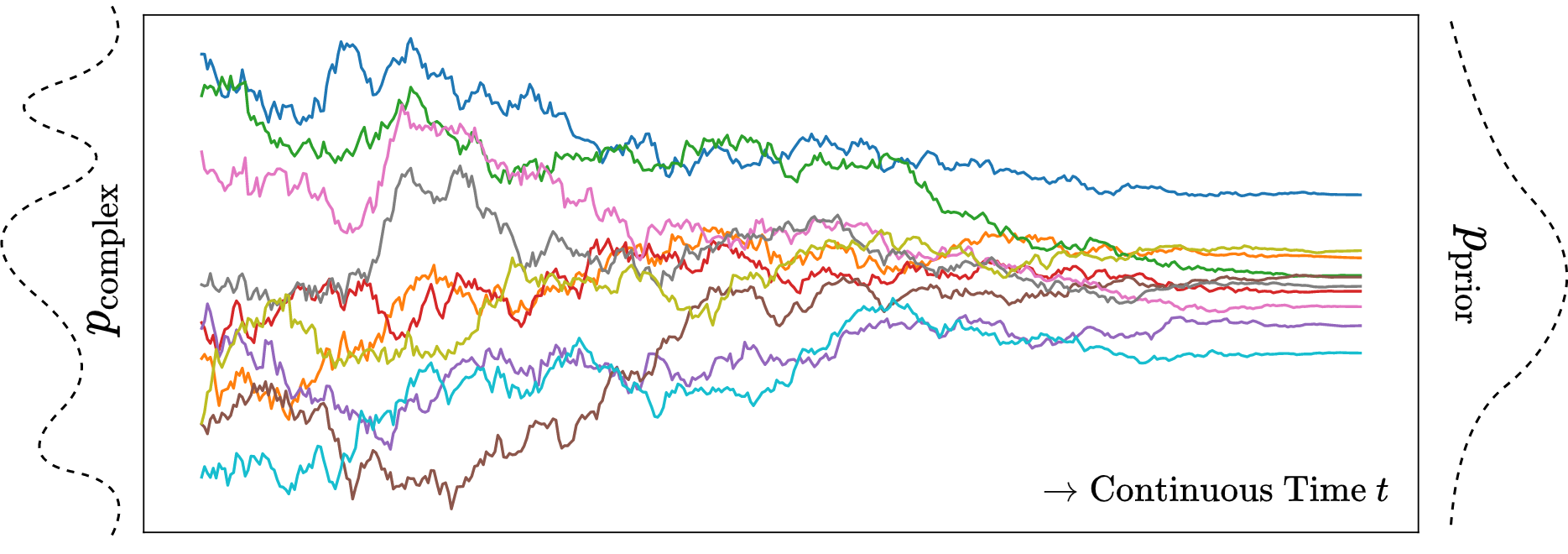
Song, Kingma, et al. (2021) (section 3.4) proposed few different choices \(\{f, g\}\) named Variance Exploding (VE), Variance Preserving (VP) and sub-VP. The one that resembles Equation 3 (discrete forward diffusion) in continuous time and ensures proper diffusion, i.e. \(\mathbf{x}(0) \sim p_{\mathrm{data}} \implies \mathbf{x}(T) \sim \mathcal{N}(0, \mathrm{I})\) is \(f(\mathbf{x}(t), t) = -\frac{1}{2}\beta(t)\mathbf{x}(t),\ g(t) = \sqrt{\beta(t)}\). This particular SDE is termed as “Variance Preserving (VP) SDE” since the variance of \(\mathbf{x}(t)\) is finite as long as the variance of \(\mathbf{x}(0)\) if finite (Appendix B of Song, Kingma, et al. (2021)). We can enforce the covariance of \(\mathbf{x}(0)\) to be \(\mathrm{I}\) simply by standardizing our dataset.
An old (but remarkable) result due to Anderson (1982) shows that the above forward diffusion can be reversed even in closed form, thanks to the following SDE
\[ d\mathbf{x}(t) = \bigg[ f(\mathbf{x}(t), t) - g^2(t) \underbrace{\nabla_{\mathbf{x}} \log p(\mathbf{x}(t))}_{\text{score }\mathbf{s}(\mathbf{x}(t), t)} \bigg] dt + g(t) d\omega(t) \tag{9}\]
Hence, the reverse diffusion is simply solving the above SDE in reverse time with initial state \(\mathbf{x}(T) \sim \mathcal{N}(0, \mathrm{I})\), leading to \(\mathbf{x}(0) \sim p_{\mathrm{data}}\). The only missing part is the score, i.e. \(\mathbf{s}(\mathbf{x}(t), t) \triangleq \nabla_{\mathbf{x}} \log p(\mathbf{x}(t))\). Thankfully, we have already seen how score estimation works and that is pretty much what we do here. There are two ways, as explained in my blog on score models. I briefly go over them below in the context of continuous SDEs:
1. Implicit Score Matching (ISM)
The easier way is to use the Hutchinson trace-estimator based score matching proposed by Song et al. (2020) called “Sliced Score Matching”.
\[ J_{\mathrm{I}}(\theta) = \mathbb{E}_{\mathbf{v}\sim\mathcal{N}(0, \mathrm{I})} \mathbb{E}_{\mathbf{x}(0)\sim p_{\mathrm{data}}} \mathbb{E}_{\mathbf{x}(0 \lt t \leq T)\sim q(\cdot\vert \mathbf{x}(0))} \bigg[ \frac{1}{2} \left|\left| \mathbf{s}_{\theta}(\mathbf{x}(t), t) \right|\right|^2 + \mathbf{v}^T \nabla_{\mathbf{x}} \mathbf{s}_{\theta}(\mathbf{x}(t), t) \mathbf{v} \bigg] \]
Very similar to NCSN, we define a parametric score network \(\mathbf{s}_{\theta}(\mathbf{x}(t), t)\) dependent on continuous time/scale \(t\). Starting from data samples \(\mathbf{x}(0)\sim p_{\mathrm{data}}\), we can generate the rest of the forward chain \(\mathbf{x}(0\lt t \leq T)\) simply by executing a solver (refer to Equation 8) on the SDE at any required precision (discretization).
2. Denoising Score Matching (DSM)
There is the other “Denoising score matching (DSM)” way of training \(\mathbf{s}_{\theta}\), which is slightly more complicated. At its core, the DSM objective for continuous diffusion is a continuous analogue of the discrete DSM objective.
\[ J_{\mathrm{D}}(\theta) = \frac{1}{T} \sum_{t=1}^T p(t) \mathbb{E}_{\mathbf{x}(0),\ \mathbf{x}(t)} \left[ \vert\vert \mathbf{s}_{\theta}(\mathbf{x}(t), t) - {\color{blue}\nabla_{\mathbf{x}(t)} \log p(\mathbf{x}(t)\vert \mathbf{x}(0))} \vert\vert^2 \right] \]
Remember that in case of continuous diffusion, we never explicitly modelled the reverse conditionals \(p(\mathbf{x}(t)\vert \mathbf{x}(0))\). The reverse diffusion was defined rather implicitly (Equation 9). Hence, the quantity in blue, unlike its discrete counterpart, isn’t very easy to compute in general. However, due to Särkkä and Solin (2019) there is an easy closed form for it when the drift function \(f\) is affine in nature. Thankfully, our specific choice of \(f(\mathbf{x}(t), t)\) is indeed affine.
\[ p(\mathbf{x}(t)\vert \mathbf{x}(0)) = \mathcal{N}(\mathbf{x}(t);\ \mathbf{x}(0)e^{-0.5\int_0^t \beta(s)ds},\ \mathrm{I}-\mathrm{I}e^{-0.5\int_0^t \beta(s)ds}) \]
Since the conditionals are gaussian (again), its pretty easy to derive the expression for \(\nabla_{\mathbf{x}(t)} \log p(\cdot)\). I leave it for the readers to try.
Computing log-likelihoods
One of the core reasons score models exist is the fact that it bypasses the need for training explicit log-likelihoods which are difficult to compute for a large range of powerful models. Turns out that in case of continuous diffusion models, there is an indirect way to evaluate the very log-likelihood. Let’s focus on the “generative process” of continuous diffusion models, i.e. the reverse diffusion in Equation 9. What we would like to compute is \(p(\mathbf{x}(0))\) when \(\mathbf{x}(0)\) is generated by solving the SDE in Equation 9 backwards with \(\mathbf{x}(T)\sim\mathcal{N}(0, \mathrm{I})\). Even though it is hard to compute marginal likelihoods \(p(\mathbf{x}(t))\) for any \(t\), it turns out there is exists a deterministic ODE (Ordinary Differential Equation) against the SDE in Equation 9 whose marginal likelihoods match that of the SDE for every \(t\)
\[ \frac{d\mathbf{x}(t)}{dt} = \bigg[ f(\mathbf{x}(t), t) - g^2(t) \underbrace{\nabla_{\mathbf{x}} \log p(\mathbf{x}(t))}_{\approx\ \mathbf{s}_{\theta}(\mathbf{x}(t), t)} \bigg] \triangleq F(\mathbf{x}(t), t) \]
Note that the above ODE is essentially the same SDE but without the source of randomness. After learning the score (as usual), we simply drop-in replace the SDE with the above ODE. Now all thanks to Chen et al. (2018), this problem has already been solved. It is known as Continuous Normalizing Flow (CNF) whereby given \(\log p(\mathbf{x}(T))\), we can calculate \(\log p(\mathbf{x}(0))\) by solving the following ODE with any numerical solver for \(t = T \rightarrow 0\)
\[ \frac{\partial}{\partial t} \log p(\mathbf{x}(t)) = - \mathrm{tr}\left( \frac{d}{d\mathbf{x}(t)} F(\mathbf{x}(t), t) \right) \]
Please remember that this way of computing log-likelihood is merely an utility and cannot be used to train the model. A more recent paper (Song, Durkan, et al. 2021) however, shows a way to train SDE based continuous diffusion models by directly optimizing (a bound on) log-likelihood under some condition, which may be the topic for another article. I encourage readers to explore it themselves.
References
Citation
@online{das2021,
  author = {Das, Ayan},
  title = {An Introduction to {Diffusion} {Probabilistic} {Models}},
  date = {2021-12-04},
  url = {https://ayandas.me/blogs/2021-12-04-diffusion-prob-models.html},
  langid = {en}
}